REGISTRO DOI: 10.5281/zenodo.11085989
Emerson Charles do Nascimento Marreiros1
Esrom José Galvão do Nascimento2
Resumo
O problema de planejamento de caminhos tem sido estudado há muito tempo. Nesta nota, determinamos analiticamente e computacionalmente a estrutura para a fronteira do Diagrama de Voronoi em um determinado caso não linear (formato de obstáculo): um obstáculo circular e dois pontos geradores. Avaliamos e mostramos as equações que determinam a fronteira e o pseudocódigo para a solução computacional. Como solução analítica, encontramos as equações cujo zero é o ponto da fronteira. Como Solução computacional, usamos o método Newton-Raphson. Além disso, traçamos a fronteira em alguns casos diferentes, alterando os seguintes parâmetros: centro do círculo e a localização dos pontos geradores.
Palavras-chaves: Diagrama de Voronoi, Obstáculo Circular, Planejamento de Caminho.
1. Introduction
The Voronoi diagram is widely studied since 1854, [1]. In the two dimensional case it can be intuitively defined as: given a finite set of points in R2, that can be called generating points, the Voronoi diagram of these points is a collection of regions, each one related to a generating point. All points that lie inside one region are closer to its generating point than to any other generating point. Also, the points that belong to the boundaries between two regions have the same distance from their generating points.
Many applications of Voronoi diagram can be found in the literature. In [2] the authors present the allocation problem in a heterogeneous space Voronoi diagram and this work also offers a good survey on allocation problems using Voronoi diagrams. An application in deep learning models in biomedicine can be found at [3]. In [4] Voronoi diagram is used to predict travel time. Another application that appears in [5] uses Voronoi diagram for internet of things. Also an application towards cost-effective 3D printing can be seen in [6].
Another field of application which is very important and actual is related to path planning as can be seen in [7], [8], [9], [10], [11]. In the literature it is not uncommon to find results about Voronoi diagram with poligonal obstacles or without obstacles. All the cited articles deal with the obstacles using approximations, which can be its convex hull, for example. Approximations of the obstacles are commonly used however, according to [12], a good approximation of an obstacle can be computationally expensive.
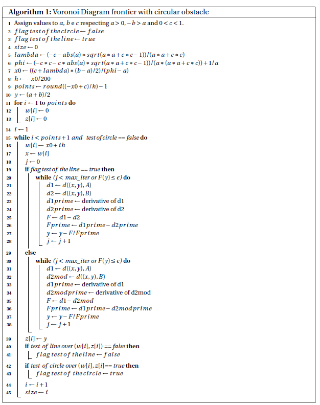
In this work a motivational example is described in order to show an application for this work. Figure 1 displays the situation with a circular obstacle to which the proposed algorithm of this work has been constructed. In war times, the mankind develops many tools and solutions for problems that have not yes been produced. Our motivational problem correspond to one application for the Voronoi diagram frontier in a war situation. We can think about one application for our result as been the best choice for a humanitarian corridor, which means to choose a corridor where refugees can go out from a city with the most safe way into a war. Such corridor is represented by the Voronoi diagram frontier. The generating points represent the location of the closest enemies from the humanitarian corridor. In this situation, the goal for the refugees can be considered to take on the minimum possible risk which means to walk over the Voronoi diagram frontier. Such way leaves the refugees over points with the same distance for the generating points. Initially, the refugee must run to the Voronoi diagram frontier. Due to the existence of the obstacle, the Voronoi diagram frontier of this work has nonlinear components (see Section 3.1).
In this note we present the algorithm that builds the frontier of Voronoi diagram with two generating points and a circular obstacle. It is important to explicit the frontier between two generating points with a circular obstacle between them because it gives the benefit to know where to move aiming at staying at the same distance of both, which configures a path planning problem. The definition of a Voronoi diagram edge, can be found in [13]. The set of all edges of Voronoi diagram correspond to the its frontier in this note.
The first contribution presented is making explicit the coordinates of the points of interest, which means having their exact location, avoiding the use of approximations. The second contribution is the algorithm that uses the distances between the points of interest and its derivatives in the Newton-Raphson method in order to generate as many points of the Voronoi diagram frontier adressed in this work as one wants. The third contribution is the frontier itself.
2. Material and Methods
Inordertosolvetheproposedproblem,theexactcoordinatesofthemainpointsQ1,Q2,Q3,Q4,Q5,Q6 and D were calculated. After that, the distances between these points were computed and also their derivatives.
With all the calculations done, they were put at the proposed algorithm. As the Voronoi diagram frontier of this work is not linear, the algorithm uses the Newton Raphson method in order to compute the frontier points. The algorithm was used to solve an instance of the motivational example of humanitarian corridor. The solution gives the frontier of Voronoi diagram which is also the path that has to be made aiming at staying at the same distance from the two generating points which at the example represent the closest enemies.
3. Theory and Calulations
3.1. Graphical representation and coordinates
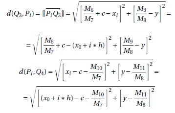
The Figure 1 shows the main points that are used to determine the Voronoi diagram frontier.
A = (0,a) and B = (0,b) are the generating points and the point C = (c,0) is the center of the circular obstacle with the following constraints a > 0,b < 0,−b > a and 0 < c < 1. The coordinates ofQ2 are such that the line segmentCQ2 is orthogonal to the line segment AQ2. In the condition that we do not have obstacle the frontier of the Voronoi diagram is the line A = (0,a) and B = (0,b) are the generating points and the point C = (c,0) is the center of the circular obstacle with the following constraints a > 0,b < 0,−b > a and 0 < c < 1. The coordinates ofQ2 are such that the line segmentCQ2 is orthogonal to the line segment AQ2. In the condition that we do not have obstacle the frontier of the Voronoi diagram is the line ![]() which is the bisector of points A and B. However, in our case many points of the frontier are out of this line. When an object or a person is making a path over the bisector of points A and B going towards the obstacle, there is a last point over the bisector that belongs to the Voronoi frontier and in this work this point is named D.
which is the bisector of points A and B. However, in our case many points of the frontier are out of this line. When an object or a person is making a path over the bisector of points A and B going towards the obstacle, there is a last point over the bisector that belongs to the Voronoi frontier and in this work this point is named D.
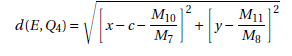
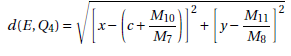
Taking E = (x,y) as a point at the frontier, the coordinates of Q3 and Q4 are such that line segments EQ3 and EQ4 are orthogonal to line segments CQ3 and CQ4 respectively. Finally, the coordinates of Q5 are such that BQ5 is orthogonal to Q5C. The point Q1 will be used in the future in order to determine the frontier of the right side of the obstacle. Besides, the points Q1,Q2,Q3,Q4 and Q5 are over the circle. In addition they are important to find the points over the frontier.
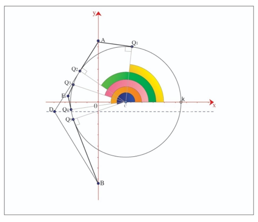
Figure 1: Main points – frontier of Voronoi diagram
In the next subsections, some propositions are announced and their demonstrations are at the appendix A.
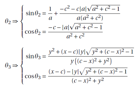
3.1.1. Coordinates of Q1 and Q2
Proposition 1. The coordinates of Q1 and Q2 are:
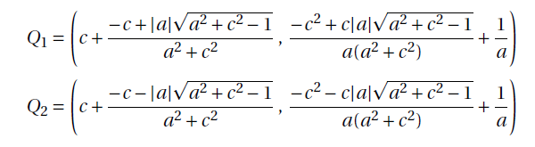
where ![]()
3.1.2. Coordinates of D
Proposition 2. The coordinates of D are:
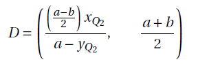
In this situation the obstacle is in between the points E and B.
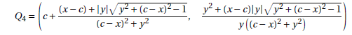
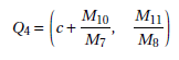
3.1.3. Coordinates of Q3 and Q4
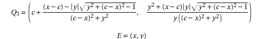
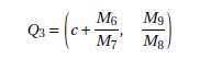
Proposition 3. Take E = (x,y) the coordinates of Q3 and Q4 are:
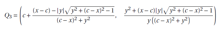
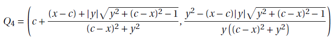
for ![]()
3.1.4. Coordinates of Q5 and Q6
The pointsQ5 andQ6 belong to the circular obstacle and their coordinates are such that BQ5 is orthogonal to CQ5 and BQ6 is orthogonal to CQ6.
Proposition 4. The coordinates of Q5 and Q6 are:
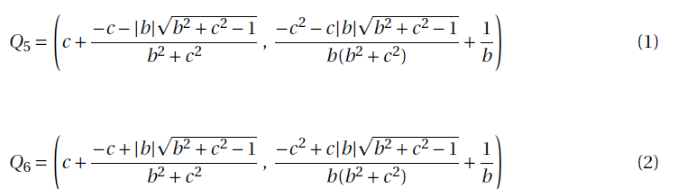
![]()
3.2. Distances
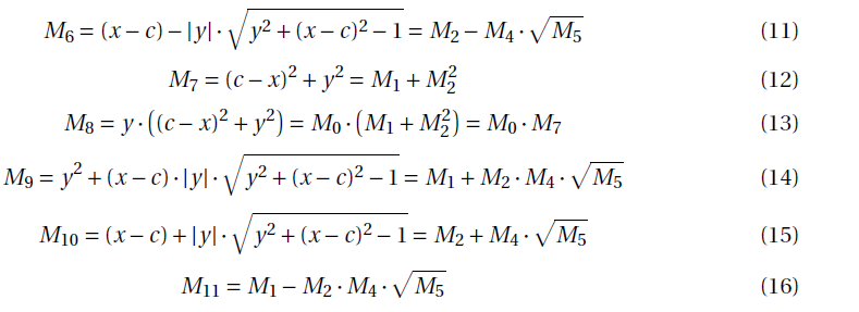
This Subsection brings the distances between the main points presented in figure 1, which are calculated using the coordinates given in Subsection 3.1. Some functions are used in this Subsection in order to shorten the equations that arise in the distances’ calculation.
3.2.1. Functions
As the functions are going to be used from the second distance that appears in this Section onwards, they are all displayed below.
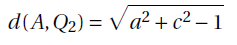
3.2.2. Computation of the euclidean distance between A and Q2.
Proposition 5. The distance between the points A and Q2 is:
3.2.3. Computation of the geodesic distance between Q2 and Q3.
Proposition 6. The distance between Q2 and Q3 is given by the length of the arc ![]() which is:
which is:

where θ3−θ2 can be calculated using
cos(θ3−θ2) = cosθ3·cosθ2+sinθ3·sinθ2,
3.2.4. Computation of the distance between Q3 and E
As the obstacle does not come between points E and Q3, it is possible to calculate the euclidean distance between them.
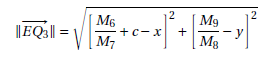
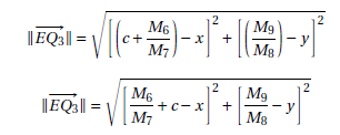
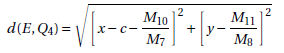
Proposition 7. The distance between the points Q3 and E is given by
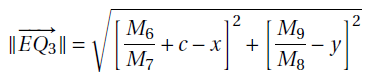
3.2.5. Computation of the distance between E and Q4
Proposition 8. The euclidean distance between the points E e Q4 is given by:
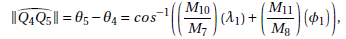
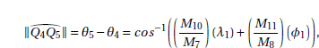
3.2.6. Computation of the geodesic distance between Q4 and Q5
Proposition 9. The geodesic distance between Q4 and Q5 is given by the length of the arc ![]()
This distance is used when the obstacle is in between the points E and B, that is, from the point E it is not possible to have direct access to point B. In this situation it is also necessary to compute the distance between Q5 and B.
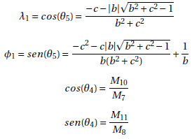
Proposition 10. The distance between Q5 and B is given by:
Now, we write about the points E from the frontier. In fact, when we will to show the points of the frontier, we will display a finite number of points denoted by Ei = (xi,yi) where xi is given by:
xi = x0+ih (18)
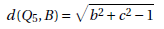
for a determined i, and h is the length of the step when moving the x-coordinate from the points Ei on the x axis towards the obstacle. Therefore the value xi of the abscissa of Ei will always be known. In order to evaluate the values for the y-coordinate from Ei we look the points over the line x = xi which can be defined by Pi = (xi,y), our goal will be the value for y that belong to the frontier, which means the values yi. Once the value of xi is known and the distances d(Q3,Pi) e d(Pi,Q4) are non linear, a numeric method can be used in order to compute the value of yi. Thus, d(Q3,Pi) and d(Pi,Q4) can be written as:
3.3. Derivatives Computations
InthisSubsectionthederivativesofthedistancesarepresentedandalsosomefunctionsthat will shorten the derivatives in order to simplify the expressions that will be used in the algorithm of Section 3.4. As the points of the frontier of the Voronoi diagram are equidistant, in order to find the coordinates of the points of its frontier, the point Pi = (xi,y) has to “move” towards the generator points A or B. Taking a look at Figure 1, the point D is the last point from which it is possible to have direct access to points A and B, meaning that the obstacle does not get in the way between D and A or D and B. On the other hand, if the point Pi = (xi,y) is at a coordinate on the right of point D considering the x axis, there are two cases to consider: Pi has direct access to point B or not. These situations are described and analyzed below.
First situation: the point Pi doesn’t have direct access to point A
In this situation, the geodesic from Pi to A is the sum of the distance from Pi to Q3 which belongs to the obstacle (circle) plus a distance fromQ3 towards the pointQ2, which corresponds to the size of the arc between these points and finally plus the distance from Q2 to A. On the other hand, Pi has direct access to B. The values of A = (0,2),B = (0,−5) and C = (0.5,0) can be used as an example of this situation. As the Voronoi frontier points are at the same distance from generation points A and B, D(Pi) can be represented as:
D(Pi) = d(A,Q2)+d(Q2,Q3)+d(Q3,Pi)−d(Pi,B). (19)
The Figure 2 shows this situation
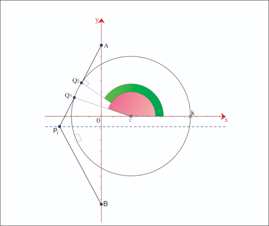
Figure 2: Geodesic distances: d(A,Pi) =d(Pi,B)
Second situation: the point Pi doesn’t have direct access neither to the point A nor to the point B.
The values of A = (0,1),B = (0,−1.3) and C = (0.5,0) can be used as an example of this situation. The calculation of the geodesic from Pi to B is analogous to that of the first situation. This geodesic is the sum of the distance from Pi to Q4 plus the size of the arc from Q4 to Q5 plus the sum of the distance from Q5 to B. So,
D(Pi)(y) = d(A,Q2)(y)+d(Q2,Q3)(y)+d(Q3,Pi)(y)−£d(Pi,Q4)(y)+d(Q4,Q5)(y)+d(Q5,B)(y).
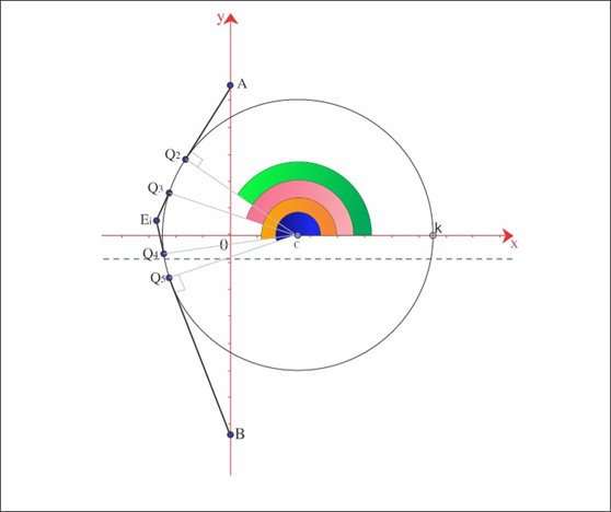
Figure 3: Second Situation
As the Newton-Raphson method is used to find the coordinate of the y axis for each xi in Pi = (xi,y), the derivatives of the distances related to situations 1 and 2 are needed.
Derivative related to the first situation
D′(Pi)(y) = d′(A,Q2)(y)+d′(Q2Q3)(y)+d′(Q3,Pi)(y)−d′(Pi,B)(y) (21)
Derivative related to the second situation:
D′(Pi) = d′(A,Q2)(y)+d′(Q2,Q3)(y)+d′(Q3,Pi)(y)−
−£d′(Pi,Q4)(y)+d′(Q4,Q5)(y)+d′(Q5,B)(y)¤ (22)
Equations 19 and 21 are used when it’s the case of the first situation and equations 20 and 22 are used in the second situation. So, for each fixed value i and taking j as the index of the Newton Raphson iterations, with z0 = yi−1, the iterations are:
![]() , for a fixed value of i. (23)
, for a fixed value of i. (23)
After finishing the iterations for a fixed value of i, the last value of zj is the value of yi. Thus, the value of the coordinates of the point of the Voronoi frontier E(xi,yi) related to a specific value of i are known.
3.4. Algorithm
At the beginning of this Subsection the main parts of the algorithm are explained. After that, the algorithm to find points belonging to the frontier of the Voronoi diagram addressed in this work is presented.
3.4.1. Initialization
The initialization part of the algorithm is at lines 1 to 13. The values of a,b and c are setted up.
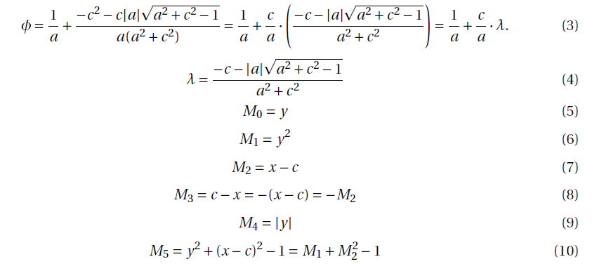
In the algorithm, two point-set problems need to be answered. Considering the line that pass by the points B and Q5, the first point-set problem consists on knowing if a determined point is below this line (which in the algorithm is represented by the test of line). The second pointset problem consists on to verify if a point is inside the circular obstacle (in the algorithm it is represented by the test of circle). Still in the initialization part, the equations for calculating the lambda,phi,x0 and h values are provided.
3.4.2. First situation
The first situation is at instructions from line 19 to line 27 of the algorithm. Given the value of xi, at the end of these instructions, the value of the yi coordinate is obtained.
3.4.3. Second situation
The second situation is presented at instructions from line 28 to line 36 of the algorithm. Given the value of xi, at the end of these instructions, the value of the yi coordinate is obtained.
3.4.4. Tests
At lines from 40 to 43, two tests of set point problems are carried out over the boundary point that has just been generated. The first one, called test of line over (x,y), concerns on determine if the point (x,y) is above or below the line that connects the points B and Q5 (see Figure 3) . The second one, assign as test of the circle over (x,y), concerns on determine if the point (x,y) is inside or outside from the circle (obstacle).
3.4.5. Stopping criterion
In the algorithm there is a stopping criterion when applying the Newton-Raphson method which consists of maximum number of iterations named max_iter or if the function is close to zero . This parameter is not greater than 5. This occurs because the algorithm converges rapidly.
4. Results and Discussions
In this paper the problem of finding the frontier of the Voronoi diagram with two generating points and a circular obstacle has been studied in light of an object that is moving towards the obstaclebutkeepingthesamedistancefromthegeneratingpoints. Inordertofindafinitenumber of points which describe the frontier, the coordinates of some specific points (main points) were defined and evaluated. After that, the values of the distances (sometimes the geodesic distances)werecalculated. Thesedistancesarefunctionsofonevariable y. TheNewthon-Raphson method was used in the algorithm, which implied the need of the derivatives from these distances.
The proposed algorithm, which generates several points of the Voronoi diagram frontier, uses all information from the previous Sections of this work. From the points generated by the algorithm it can be observed that the frontier has a curved aspect with an upward trajectory in relation to the axis of the ordinates. The Figure 4 has three subfigures, the left and middle ones relating to the first situation. The difference between these subfigures is that for different coordiantes of A and B the frontier may or may not touch the obstacle. The right subfigure is related to the second situation. The first and the second situations are described at 3.3. The blue part in the figures refers to the points at the middle line between the points A and B (at this blue part the frontier is still a line).
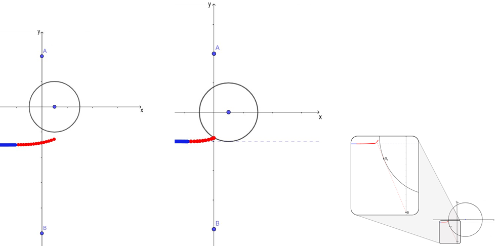
Figure 4
The results of this work can be used in self-driving car trajectories, self-driving robots and autonomous underwater vehicles trajectories which are some examples.
5. Conclusion
In this work it became clear how the frontier of the Voronoi diagram for only two points and a circular obstacle can be generated, solving the path planning towards the obstacle. The next step is either increase the number of points with only one circular obstacle or increase the number of circular obstacles and only two generator points. The problem with many obstacles and many points seems to be really a big challenge.
Appendix A. Demonstrations of Propositions from Section 3.2
Proposition 5 The distance between the points A and Q2 is:
Demonstration:
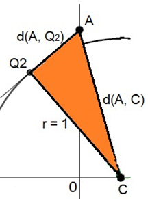
Figure A.5: Distance between A and Q2
Created by the author
In order to determine the euclidean distance between A and Q2, the Pythagorean theorem is used.
A = (0,a),C = (c,0) and r = 1. (A.1)
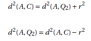
The distanced(A,C) must be available in order to permit calculation of the distance d(A,Q2).
Therefore:
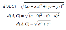
Once the distance d(A,C) has been obtained, the Pytagorean theorem can be used again in order to determine the distance d(A,Q2).
Proposition 6 The distance between Q2 and Q3 is given by the length of the arc ![]()
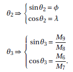
Demonstration: The functions sin(·) and cos(·) of θ2 and θ3 respectively, can be represented using the functions φ,λ and Mi, com i = 6,…,9:
Making the appropriate substitutions, equation 17 is found.
Proposition 7 The distance between the points Q3 and E is given by:
Demonstration:
The coordinates of points Q3 and E are, respectively:
Using functions Mi, with i = 6,…,9, the coordinates of M3 can be rewritten as:
The norm of the vector EQ−−→3 is the euclidean distance between the points Q3 and E. Thus:
Proposition 8
The euclidean distance between the points E e Q4 is given by:
Demonstration:
Given the coordinates of the points:
E = (x, y)
e
Rewriting the coordinates of Q4 using the functions Mi, com i = 7,8,10,11,··· ,11. it becomes:
Right now, we have just demonstrated the distance between the points E and Q4
Thus, we obtain:
Proposition 9 The geodesic distance between Q4 and Q5 is given by the length of the arc ![]()
Demonstration:
Proposition 10 The distance between Q5 and B is given by:
Demonstration:
This proof is analogous to the proof of the distance between points A and Q2.
References
- H. Brody, M. Rip, P. Vinten-Johansen, N. Paneth, S. Rachman, Map-making and mythmaking in broad street: The london cholera epidemic, 1854, Lancet 356 (2000) 64–8. doi:10.1016/S0140-6736(00)02442-9.
- X. Feng, A. Murray, Allocation using a heterogeneous space voronoi diagram, Journal of Geographical Systems 20 (07 2018). doi:10.1007/s10109-018-0274-5.
- F. J., S. W. R. J., B. M., A Voronoi Diagram-Based Representation of Ligand-Binding Sites in Proteins for Machine Learning Applications., 2021, pp. 299–312. doi:https://doi.org/ 10.1007/978-1-0716-1209-5_17.
- K. Adhinugraha, D. Taniar, T. Phan, R. Beare, Predicting travel time within catchment area using time travel voronoi diagram (ttvd) and crowdsource map features, Information Processing & Management 59 (3) (2022) 102922. doi:https://doi.org/10.1016/j.ipm.2022.102922.URL https://www.sciencedirect.com/science/article/pii/S0306457322000462
- S. Wan, Y. Zhao, T. Wang, Z. Gu, Q. H. Abbasi, K.-K. R. Choo, Multi-dimensional data indexing and range query processing via voronoi diagram for internet of things, Future Generation Computer Systems 91 (2019) 382–391. doi:https://doi.org/10.1016/j.future.2018.08.007.URL https://www.sciencedirect.com/science/article/pii/S0167739X18311956
- A. Zheng, S. Bian, E. Chaudhry, J. Chang, H. Haron, L. You, J. Zhang, Voronoi diagram and monte-carlo simulation based finite element optimization for cost-effective 3d printing, Journal of Computational Science 50 (2021) 101301. doi:https://doi.org/10.1016/j. jocs.2021.101301.URL https://www.sciencedirect.com/science/article/pii/S187775032100003X
- B. B. K. Ayawli, X. Mei, M. Shen, A. Y. Appiah, F. Kyeremeh, Mobile robot path planning in dynamic environment using voronoi diagram and computation geometry technique, IEEE Access 7 (2019) 86026–86040. doi:10.1109/ACCESS.2019.2925623.
- S. Sedighi, D.-V. Nguyen, P. Kapsalas, K.-D. Kuhnert, Implementing voronoi-based guided hybrid a in global path planning for autonomous vehicles, in: 2019 IEEE Intelligent Transportation Systems Conference (ITSC), 2019, pp. 3845–3852. doi:10.1109/ITSC.2019.8917427.
- J. Hu, H. Niu, J. Carrasco, B. Lennox, F. Arvin, Voronoi-based multi-robot autonomous exploration in unknown environments via deep reinforcement learning, IEEE Transactions on Vehicular Technology 69 (12) (2020) 14413–14423. doi:10.1109/TVT.2020.3034800.
- K.-C. Huang, F.-L. Lian, C.-T. Chen, C.-H. Wu, C.-C. Chen, A novel solution with rapid voronoi-based coverage path planning in irregular environment for robotic mowing systems, International Journal of Intelligent Robotics and Applications 5 (12 2021). doi: 10.1007/s41315-021-00199-8.
- Y. Shi, L. Zhang, S. Dong, Path planning of anti ship missile based on voronoi diagram and binary tree algorithm, Defence Science Journal 69 (4) (2019) 369–377. doi:10.14429/dsj.69.14062.URL https://publications.drdo.gov.in/ojs/index.php/dsj/article/view/ 14062
- H. Alt, O. Cheong, A. Vigneron, The voronoi diagram of curved objects, Discrete & Computational Geometry 34 (2005) 439–453. doi:10.1007/s00454-005-1192-0. URL https://doi.org/10.1007/s00454-005-1192-0
- A. Dobrin, A review of properties and variations of voronoi diagrams.
1Mestre em Modelagem Matemática e Computacional pela Universidade Federal da Paraíba – UFPB.
ORCID: http;//orcid.org/0009-0006-0374-7056
2Graduando-se em Bacharelado em Sistemas de Informação pela Faculdade UNINASSAU-Polo Parnaíba-PI.
ORCID: http;//orcid.org/0009-0004-2561-3118