REGISTRO DOI: 10.5281/zenodo.12629754
Neiton Silva Machado1
Felipe Rodrigues Freire2
Karla Dos Santos Melo De Sousa3
Adriano Victor Lopes Da Silva4
Daniel Mariano Leite5
Julio Cesar Ferreira Melo Junior6
ABSTRACT
The objective of this study was to adjust mathematical models to the growth of loofah (Luffa Cylindrica (L.) M. Roem.) seedlings. To do this, it was necessary to analyze the morphological variables of the crop, such as the length of the main branch, number of leaves, diameter of the stem base and leaf area. Furthermore, the relationship between these variables and the accumulated degree days (ADD) was verified. The water, total, fixed and volatile solids contents of the aerial part of the crop were also analyzed, as well as the elemental composition of carbon, hydrogen and oxygen. The experiment was carried out in a screened nursery with 50% shading. Five seedlings from each accession were sampled every 3 days, totaling five replications, until the end of the cycle. Among the adjusted mathematical models, the 4-parameter Sigmoid model presented the highest adjusted R2 for the dry mass variable in relation to ADD, reaching 0.870. The point of greatest growth of the crop, followed by stability in the number of leaves and dry mass, was reached at 346.60 ADD.
Keywords: mathematical model, correlation, curcubitaceae, plant fiber, Luffa Cylindrica (L.) M. Roem
RESUMO
O objetivo deste estudo foi ajustar modelos matemáticos ao crescimento de mudas de bucha vegetal (Luffa Cylindrica (L.) M. Roem.). Para isso, foi necessário analisar as variáveis morfológicas da cultura, como comprimento da rama principal, número de folhas, diâmetro da base do caule e área foliar. Além disso, foi verificada a relação entre essas variáveis e os graus dia acumulados (GDA). Também foram analisados os teores de água, sólidos totais, fixos e voláteis da parte aérea da cultura, assim como a composição elementar de carbono, hidrogênio e oxigênio. O experimento foi realizado em um viveiro telado com 50% de sombreamento. Foram amostradas cinco mudas de cada acesso a cada 3 dias, totalizando cinco repetições, até o final do ciclo. Entre os modelos matemáticos ajustados, o modelo Sigmoide 4 parâmetros apresentou o maior R2 ajustado para a variável de massa seca em relação aos GDA, alcançando 0,870. O ponto de maior crescimento da cultura, seguido pela estabilidade do número de folhas e massa seca, foi atingido em 346,60 GDA.
Palavras-chave: modelo matemático, correlação, curcubitaceae, fibra vegetal, Luffa Cylindrica (L.) M. Roem
RESUMEN
El objetivo de este estudio fue ajustar modelos matemáticos al crecimiento de plántulas de lufa (Luffa Cylindrica (L.) M. Roem.). Para ello fue necesario analizar las variables morfológicas del cultivo, como longitud de la rama principal, número de hojas, diámetro de la base del tallo y área foliar. Además, se verificó la relación entre estas variables y los grados día acumulados (GDA). También se analizó el contenido de agua, sólidos totales, fijos y volátiles de la parte aérea del cultivo, así como la composición elemental de carbono, hidrógeno y oxígeno. El experimento se llevó a cabo en un vivero cubierto con 50% de sombra. Se muestrearon cinco plántulas de cada accesión cada 3 días, totalizando cinco repeticiones, hasta el final del ciclo. Entre los modelos matemáticos ajustados, el modelo Sigmoide de 4 parámetros presentó el mayor R2 ajustado para la variable masa seca en relación al GDA, alcanzando 0,870. El punto de mayor crecimiento del cultivo, seguido de estabilidad en el número de hojas y masa seca, se alcanzó en 346,60 GDA.
Palabras Clave: modelo matemático, correlación, curcubitáceas, fibra vegetal, Luffa Cylindrica (L.) M. Roem
INTRODUCTION
Loofah, introduced to Brazil by Portuguese colonizers, became popular in several states across the country. Although there are no official data on commercial plantations, the city of Bonfim, in Minas Gerais, stands out as the main national producer, with an annual harvest of 100 thousand dozens (CARVALHO, 2007). According to the aforementioned author, growing loofah through seedlings brings numerous advantages compared to directly planting the seeds in the soil. This practice allows prior selection of plants, provides better soil preparation, resulting in greater seedling growth and more effective control of diseases and pests in the initial stages of cultivation. Furthermore, the germination rate is improved due to more efficient irrigation in the nursery, resulting in healthy, well-developed plants, thus reducing replanting and irrigation costs in the field.
Vegetable loofah plays a fundamental role in the agroecological products market, thanks to the versatility of its natural fibers and its use in various sectors of the agroindustry (MAIA et al., 2019). It is important to highlight that, at the 27th edition of COP (United Nations Conference on Climate Change), Brazil reaffirmed its commitment to sustainability, without neglecting its development. To continue on this path, it is essential to invest in research and improve the techniques used. Therefore, the production of vegetable loofah in the Brazilian semi-arid region faces specific challenges, such as soil salinity and water scarcity. In semi-arid regions, irrigation water can be saline (EC > 1.0 dS/m) and harm the production of loofah. In case of suspected salinity, soil analysis and application of appropriate management techniques are suggested to minimize the negative effect of salinity.
Marouelli, Da Silva and Lopes, (2013) state that to overcome these challenges, loofah producers in the Brazilian semi-arid region must adopt sustainable management practices, such as the use of drip irrigation, especially when associated with the use of soil cover with black plastic, which has been advantageous in the production of vegetable loofah, resulting in great water savings. Furthermore, it is essential to guarantee a minimum wetted area, between 35% and 60%, so as not to limit the development of the plants’ root system and compromise production. Furthermore, the Vale do Submédio São Francisco region is also affected by environmental problems, such as desertification, which is a serious process that affects the northeastern region, and the loss of biodiversity, which is one of the country’s main environmental challenges (SA, et al 2009)
In this sense, the use of mathematical models to estimate seedling growth as a function of accumulated degree days – ADD can be a crucial tool in predicting plant development. These models describe the system through mathematical equations that require specific data to be adjusted. Mathematical models can be classified as linear or non-linear, depending on the equations they represent (GAONA, 2006).
A sigmoidal model is characterized by an S-shaped sigmoid function, with non-linear parameters and a random component following a probability distribution. These models are widely used in various areas of knowledge, such as epidemiology, agronomy, chemistry, engineering, neural networks and biomedical sciences. They are used to describe processes in which the relationship between a response variable Y and an explanatory variable X is represented by a curve that initially has an increasing growth rate, reaches an inflection point and then decreases, asymptotically approaching a value final, known in some applications as bearing capacity (CARMO, 2022).
Non-linear models have been widely used by several authors to describe the growth of individuals (Souza et al., 2007; Melo Júnior et al., 2015; Veloso et al., 2016; Azarias, et al., 2023; Fernandes et al., 2023; Machado et al., 2023; Silva et al., 2023 e Vilas Boas, et al., 2023). These models have parameters with biological significance, contributing to a better understanding of the growth process. However, choosing the ideal model is not always a simple task. There are several mathematical criteria used as evaluators to determine which model offers the best fit. These include coefficient of determination (R2), adjusted coefficient of determination (R²aj), root mean square residual (MSR), mean absolute deviation (MAD), asymptotic standard deviation (ASD), asymptotic index (AI) , the Akaike information criterion (AIC) and the Bayesian information criterion (BIC).
Given the above, the main objective of this study was to adjust sigmoid and 3D-plane mathematical models to the growth of loofah seedlings (Luffa Cylindrica (L.) M. Roem.). For this, it was necessary to quantify the morphological variables of the crop, such as length of the main branch, number of leaves, diameter of the stem base and leaf area. Furthermore, the correlation between these observed variables and the accumulated degree days (ADD) was calculated, as well as the water content and total, fixed and volatile solids content of the aerial part of the crop were determined. Finally, the estimation of the elemental composition of carbon, hydrogen and oxygen of the aerial part of the crop was also carried out.
MATERIAL AND METHODS
The study was carried out at the Agricultural Sciences Campus of the Federal University of Vale do São Francisco (Univasf), located in Petrolina, Pernambuco, Brazil. The experiment conditions included a screened nursery with 50% shading, located at geographic coordinates of 9º 19′ 15″S and 40º 32′ 40″W. The region has a BSh’ climate classification, characterized as very hot steppe drought, according to Köppen’s proposal (MELO JÚNIOR, et al., 2015).
Feedstock
For the production of seedlings, seeds of 2 genotypes of Loofah Vegetal (Luffa Cylindrica (L.) M. Roem) were acquired. Genotype 1 was collected in a residential area close to Condomínio Vivendas do Rio, in Petrolina, Pernambuco. Genotype 2 was found at country house of Luis Nelinho, located in Lagoa Grande, Pernambuco.
Seedling production
The 500 mL disposable cups were selected as containers for the production of seedlings, being filled with organic compost provided by the Olericulture and Agroecology Nucleus (NOA) at Univasf. This strategic choice guaranteed the quality and success of the plant cultivation process.
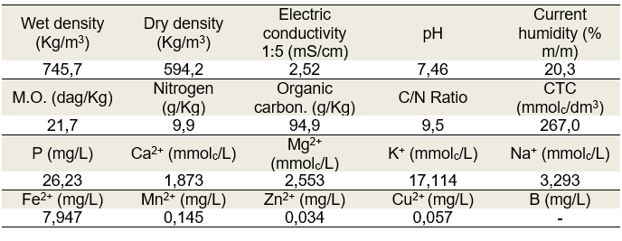
We developed an innovative compost from several layers of crushed grass residues, together with goat and cattle manure, both rich in essential nutrients for plant growth. Additionally, we added 1 kg/m2 of rock powder to further enrich the substrate. The perfect combination of 30 cm of straw for 10 cm of manure resulted in a high quality compost, whose physical-chemical composition can be seen in Table 1.
Table 1 – Result of physical-chemical analyzes of the substrate (organic compound) used to produce seedlings
The sowing strategy adopted on August 31, 2023 consisted of inserting 3 seeds per container, aiming to enhance the germination rate. After seedling emergence, thinning was carried out by cutting the base of the stem of the less vigorous seedling. This procedure guaranteed the healthy development of the plants.
A total of 238 containers were used, with 119 destined for Access 1 and the other 119 for Access 2, respectively. Among the 119 cups used in each access, 60 were directly used in the analyzes (with 12 collections and 5 replications each) and the remaining 59 were used as borders.
The sub-irrigation system has a capacity of 0.2835m3, with dimensions of 1.80×2.25m in length and 0.07m in depth. The choice of sub-irrigation was based on the search for more efficient and homogeneous wetting, guaranteeing ideal humidity without causing the substrate to become waterlogged. This favors the growth and development of the seedlings. Furthermore, the use of a sheet of water as a physical barrier proved to be effective in controlling leaf-cutter ants.
Obtaining the data
For data collection, five seedlings of each sample were acquired, totaling 12 collections throughout the experiment, with an interval of 72 hours between each sampling.
Soon after collecting the samples, biometric data were recorded, including the number of leaves, the diameter of the base of the stem measured with a digital caliper and the length of the main branch measured with a measuring tape. Plant height was determined as the distance between the base of the stem and the apex of the most developed new leaf. This approach guaranteed the accuracy and quality of the results obtained.
Relative humidity and air temperature conditions were monitored in the greenhouse during sample collection, using a digital thermo-hygrometer.
After the meticulous process of biometric analysis of the seedlings, they were removed from the plastic container with the help of scissors, making a precise cut at the base of the stem to obtain the dry matter of the aerial part. After removal, the cut area was carefully washed to remove any substrate residue. The samples were then weighed on a precision scale, individually packaged in Kraft paper bags, and placed inside a forced ventilation oven. The air temperature was adjusted to 65°C and maintained for 72 hours or until the dry mass reading became constant.
The LeafArea application was used to measure leaf area. The photos were taken with the Smartphone camera positioned perpendicular to the bench, at a distance of 7 cm from the target. Furthermore, a 5 cm line was drawn next to the leaf blade as a reference. Measurements were made based on the median leaf of the main branch.
The measurement of the ambient temperature outside the roof was carried out using an automated meteorological station positioned close to the experimental area. The calculation of accumulated degree days (ADD) was based on the formula proposed by Souza et al (2007), allowing an accurate assessment of the climatic conditions in the experiment.

On what:
ADD = Accumulated degree days (ºC)
Tmax = maximum air temperature (ºC)
Tmin = minimum air temperature (ºC)
Tb = lower base temperature (ºC)
For Tb, the value of 10oC was adopted as the minimum tolerant temperature for bushing development.
Solids analysis
The analyzes of the following solids were conducted according to the guidelines of the Solid Waste and Wastewater Analysis Manual (MATOS, 2015). All crucibles were transported and handled carefully, using suitable metal tweezers, in order to avoid any interference from water, hand grease or gloves in the analyses.
Total solids
The samples were removed from the oven, where they remained at 65 ºC for more than 72 hours. Then, the material was ground in a porcelain mortar and placed in crucibles (30 mL) previously calcined. After that, weighing was carried out on the analytical balance with an accuracy of 0.0001g to obtain the mass of the dry sample (Ms). The mass of the wet sample (Mu) was obtained by weighing the material before being placed in the oven. To determine total solids, equation 2 was used.

On what:
TS = total solids (dag.kg-1 or %);
Md = mass of the dry sample at 65 ºC+ Mr (g);
Mc = mass of the container (g); It is
Mw = mass of the wet sample + Mc (g).
Fixed and volatile solids
After weighing on the analytical balance to determine the mass of the dry sample (Ms), the crucibles with the plant material were subjected to a temperature of 550 °C in the muffle furnace for 4 hours. Then, the crucibles were transferred directly to a heating plate at 100 °C, in order to avoid thermal shock and possible cracks in the containers. They were then placed in the desiccator to reach thermal equilibrium with the environment before being weighed on the analytical balance, thus obtaining the mass of the residue after combustion (Mc). Equations 3 and 4 were used to determine volatile and fixed solids.
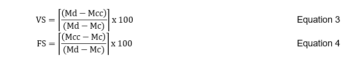
On what:
VS = volatile solids (dag.kg-1 or %);
FS = fixed solids (dag.kg-1 or %); It is
Mcc = mass of residue after combustion + Mc (g).
Elementary composition
The distribution of nutrients in Luffa Cylindrica M. Roem varies according to the part of the plant, with the leaves accumulating more nitrogen, calcium, iron and manganese, while the flowers and fruits concentrate phosphorus, potassium, magnesium, sulfur, copper and zinc (SIQUEIRA, et al. 2009). To analyze the elemental composition of the plant, the methodologies proposed by Parikh and Ghosal (2005, 2007) and suggested by Oliveira (2010) were used, which include algebraic equations based on the analysis of lignocellulosic materials.

On what:
C= Carbon content, (%)
H = Hydrogen content, (%)
O= Oxygen content (%)
FS = Fixed solids content
VS = Volatile solids content
Equations 5, 6 and 7 were developed for the analysis of solid lignocellulosic materials, taking into account the values of fixed carbon, volatile solids and ash. The results obtained presented an average absolute error of 3.21% for carbon, 4.79% for hydrogen and 3.40% for oxygen in relation to the measured values.
Adjustment and selection of mathematical models
Adjustments of five mathematical models using sigmoid curves, each with four parameters, were made to the plant growth data. The mathematical equations of the adjusted models are described below
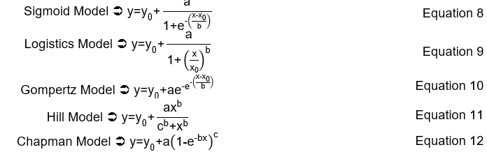
On what:
a = upper asymptote or maximum value estimated by the model;
b = model scale factor or curve displacement;
x0 or c = model inflection point;
y0 = lower asymptote or minimum value estimated by the model;
e = exponential;
y = Dependent variable;
x = Independent variable.
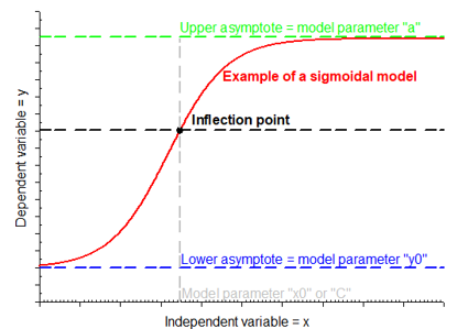
Figure 1 – Graphic illustration of the models’ behavior
Additionally, 3D models were adjusted – plans (Equation 13) with dry mass (DM) as dependent variable, and accumulated degree days (ADD), leaf area (La), stem diameter (Sd) and plant height (Ph) as independent variables.

On what:
a, b and c = model adjustment parameters;
z = Dependent variable;
x and y = Independent variables.
In the present study, we used adjusted R-squared as a mathematical evaluation metric. This metric allows us to determine how much of the variation in the dependent variable can be explained by the independent variable. The difference between adjusted R-square is that it only considers the impact of independent variables that actually influence the variation in the dependent variable. Below is highlighted the Adjusted Coefficient of Determination (R2aj) equation that was used:

On what:
(n – p) = degrees of freedom;
n = number of observations;
p = number of estimated coefficients.
Pearson’s Correlation Coefficient, also known as Product-Moment Correlation Coefficient or simply Pearson’s r, was determined by equation 15
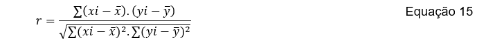
On what:

All analyzes were performed using SigmaPlot 11 and SPSS13 software.
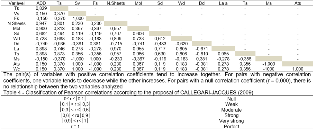
There are several similar classifications to interpret the magnitude of Pearson’s correlation coefficient (r), however the classification developed by CALLEGARI-JACQUES (2009) Table 4 was adopted in this work.
RESULTS AND DISCUSSION
Germination/emergence of Accessions/Genotypes
In the study carried out by Vadera, Pandya and Mehta (2021), it was highlighted that seed germination and overcoming dormancy represent a significant challenge for plants in the Cucurbitaceae family, due to the existence of a resistant seed coat.
During the experiment, it was found that the seeds germinated after 6 days of sowing. Accession 1 showed the emergence of 6 seedlings, while Accession 2 showed the emergence of 28 seedlings. In both genotypes, only cotyledonary leaves were present.
After 14 days of sowing, Accession 1 showed a total of 17 containers with emerging seedlings, while Accession 2 recorded 81 containers with emerging seedlings. Seedlings from both Accessions displayed primary leaves during this period.
Accession 1 was reseeded using dormancy breaking. The mechanical method applied was a small cut at the end opposite the seed hilum. However, after 7 days of reseeding, only 15 seedlings emerged. Then 7 more seedlings appeared with heterogeneity of days between emergences.
The study carried out by Primak et al. (2017) on the breaking of dormancy in loofah seeds through thermal, mechanical and chemical treatments showed that none of these methods were effective in overcoming the natural dormancy of Luffa Cylindrica L. seeds. Furthermore, the sensitivity of the loofah to salinity was evidenced, since the increase in the saline level in the irrigation water negatively impacted the germination and development of the species, with a reduction observed from 0.5 dS.m-1. (GUIMARÃES, et al. 2013).
According to the study carried out by Ramos et al. (2023), it is suggested to apply doses of 1.77 to 3 mL of Stimulate® per liter of distilled water to optimize the development of Luffa Operculata seeds. This strategy resulted in significant improvements in several aspects, such as the first emergence count, the emergence speed index, the mean emergence time, the emergence uncertainty, the number of leaves and the length of the seedlings.
Given this surprising turn of events, it was decided to discard the data from Access 1 to adjust the growth models, due to the incompatibility of the genetic factor of natural dormancy with the objectives of this study. The data from Access 2, on the other hand, proved to be adequate for the experimental analyzes proposed at the beginning of the experiment, being the only ones used.
Conducting and developing the morphology of Accession/Genotype 2 seedlings
The production of vegetable loofahs requires special care in irrigation, which can be carried out using different systems, depending on the variables present in the cultivation environment (MAROUELLI, DA SILVA and LOPES, 2013). The use of sub-irrigation to guide the seedlings was initially adopted, but problems such as excess moisture in the substrate, yellowing and withering of the leaves, and excessive development of the root system were observed. These aspects point to the need for adjustments in the irrigation technique to ensure the healthy development of plants.
Given these circumstances, it was decided to transfer the containers to a metal bench (21 days after sowing), with water being supplied daily through watering cans.
After implementing the change, it was observed over the days that the leaves returned to displaying their vibrant color and growth was reestablished. With the adoption of this new conduction system, developed specifically for the substrate used, we noticed a significant improvement in the aeration of the root zone, which resulted in an increase in gas exchange.
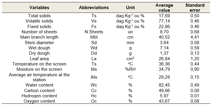
It can be seen in Table 2 that only 18% of the composition of the seedling is total solids, with an average of 77.14% volatile solids (organic part) and 22.86% fixed solids (inorganic part), in relation to the elemental composition we have the following results: carbon content around 49.66% (in general from photosynthesis); hydrogen content 5.97% (in general water); and oxygen content with 43.67% (in general from water and respiratory process). The water content in the composition of the seedlings was around 82.45%, demonstrating the importance of adequate management of the water depth for the production of quality seedlings (EMBRAPA, 2005). The leaf area of all readings was on average 26.84 cm2, with an average number of leaves between 8 and 9. The average air temperature during seedling development was around 28.28 oC, being within the ideal range that is between 22 and 35 oC (CARVALHO, 2007). The data in Table 2 reveal that only 18% of the seedling’s composition consists of total solids, with the organic part responsible for an average of 77.14% of the volatile solids and the inorganic part for 22.86% of the fixed solids. Regarding the elemental composition, we observe that the carbon content is approximately 49.66% (mainly from photosynthesis), the hydrogen content is 5.97% (mainly from water) and the oxygen content is 43 .67% (mainly from water and the respiratory process). The presence of water in the composition of the seedlings is around 82.45%, which highlights the importance of adequate management of the water depth to guarantee the production of high quality seedlings (EMBRAPA, 2005). The average leaf area was 26.84 cm2, with an average number of leaves between 8 and 9. The average air temperature during seedling development was approximately 28.28 oC, remaining within the ideal range of 22 to 35 oC recommended by Carvalho, (2007).
Table 2 – Mean values and standard errors of the analyzed variables.
Correlations between the analyzed variables
The Pearson Correlation Coefficients of the analyzed variables are included in table 3 and the classification adopted in table 4. This coefficient is a powerful statistical instrument that helps us explore the relationship between variables. With values that can vary between -1 and 1, this coefficient provides us with precise information about the intensity and direction of the joint behavior of the analyzed variables.
In short, calculating the Pearson Correlation Coefficient helps us determine the degree of correlation between two dependent variables.
The two positive correlations that stood out the most were: N.Leaves and C.Branch = 0.957 (very strong correlation), as expected the tendency for the main branch to grow in length and the number of leaves increases; and, GDA and N.Leaves = 0.947 (very strong correlation), with the accumulation of photoassimilated energy during the development of the seedling there is a tendency for the number of leaves to increase, due to the exponential growth up to the support capacity of the seedling (ideal moment for transplanting in the field).
With regard to negative correlations, the two that stood out the most were: SV and SF = -1.000 (perfect correlation), with regard to volatile solids and fixed solids, the increase in one depends directly on the decrease in the other, as solids totals are formed by organic mass (volatile solids – presence of carbon in the composition) and inorganic mass (fixed solids – mineral composition) (MATOS, 2015), therefore it was expected that the correlation would be perfect (linear dependence); and, ST and T.Water = -0.935 (very strong correlation), as the plant structure is basically formed by water and total solids, it was also expected that there would be a very strong correlation between these variables.
In Table 3 we can also highlight that of all the correlations between water content and another variable, the only correlation that presented a positive value was: T.Water and SF = 0.381 (moderate correlation), showing a certain dependence on linear growth, In other words, if the water content increases, fixed solids tend to increase, as water also acts as a transport vehicle for mineral nutrients (inorganic part), which are absorbed and transported to the aerial part of the plants. This fact corroborates the explanation by (VILAR, 2021).
Table 3 – Pearson correlation coefficient values
Mathematical models adjusted for the dependent variable Dry Mass
In the analysis of the sigmoid models presented in Table 5, it is possible to observe that they all had significant adjustments, as indicated by the adjusted R2, which ranged from 0.858 to 0.870. Among them, the highlight was the “4-parameter Sigmoid Model”, which obtained an adjusted R2 of 0.870 and all parameters with insignificant standard errors, whose p value was less than 0.0001, demonstrating that it was the best fit to the data. of accumulated degree days (ºC) in relation to the dry mass of the plant (g).
However, in the 4-parameter Chapman model a high standard error of 127.516 was observed in parameter “c” whose P value was 0.4119, indicating significance, that is, this fact compromised the adjustment of this model despite the adjusted R2 being similar to the other models.
The other models (Logistico, Gompertx and Hill) showed similar behavior to the signoid. All parameters with low standard error and p value less than 0.0001
Table 5 – Parameters of mathematical models adjusted with dependent variable Dry Mass – DM (g) and independent variable Accumulated Degree Days – ADD (ºC).
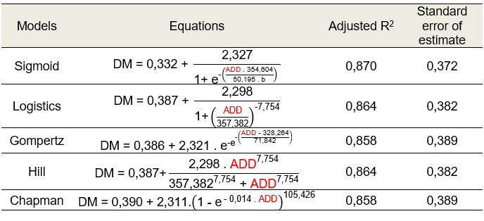
Both models presented lower and upper prediction limits for the dependent variable MS as a function of the independent variable GDA in the range of 0.3 to 2.3 as it can be seen that the “a” parameters of both models were 2.327; 2,298; 2.321 and 2.311 while the value of y0 was 0.332; 0.387; 0.386; 0.387 and 0.390, respectively. However, when observing the parameter “b” which represents the scale factor of the models, that is, the displacement of the curves, they showed great variation in numerical values, 50.195; 7,754; 71,842; 7.754 and -0.014, respectively. The inflection point of the models, that is, the point where there is a change in the direction of curvature, was 354.604; 357,382; 328,264; 357,382 and 105,426, respectively. All models presented a similar inflection point except for the Chapman model (GDA = 105.426) whose justification lies in the high standard error of the parameter as already mentioned.
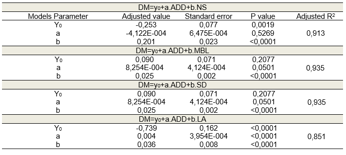
The 2D models with sigmoid curves for simulating plant growth presented a good fit for the dependent variable MS in relation to the independent variable ADD, with R2ajs equal to 0.870; 0.864; 0.858; 0.864 and 0.858, respectively. While the flat 3D models (Table 5) presented an adjusted R2 of 0.913; 0.935; 0.935 and 0.851, for dependent variable MS and independent variables ADD and NF; ADD and CPR; ADD and DC; ADD and AF, respectively.
HONORATO et al. (2014) observed, for the adjustment of the expolinear growth model to data on total dry biomass (aerial and root parts) accumulated from cowpea, cultivar BRS Pujante, an adjusted coefficient of determination (R2 ajs) equal to 0.9654. MOURA et al. (2011) using the expolinear growth model to simulate the growth of cowpea, cultivar Guaribas, for two cultivation systems and observed that the model adjustments presented R2 ajs equal to 0.9967 and 0.9808, respectively, for the exclusive and intercropped cultivation. TEI et al. (1996a), using the expolinear model to simulate the growth of lettuce, onion and beet plants, obtained R2 ajs values equal to 0.993, 0.997 and 0.996, when considering the ADD. LYRA et al. (2003), with the objective of adjusting growth simulation models for the lettuce crop, obtained values of R 2 ajs equal to 0.9985, 0.9941 and 0.9981, when considering the ADD.
GRAPPADELLI (2005), applying the expolinear model to define the peak of cytokinesis in apple fruit, observed, respectively, the values 0.2 g fruit-1 d-1, 0.038 g g-1 °d-1 and 74 d for “a” , “b” and “x0”.
The graphical representation of the correlation between the dry mass values observed in the laboratory and those estimated by the equations in table 4 are illustrated in figure 2.
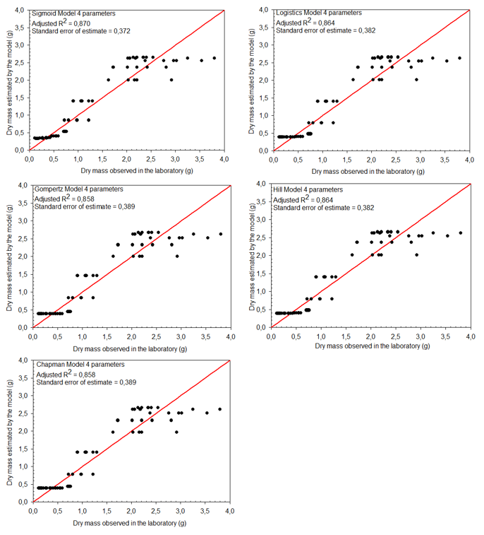
Figure 2 – Correlation of Dry Mass (g) predicted by the adjusted models with Dry Mass observed in the laboratory: A) Sigmoid 4 parameters; B) Logistics 4 parameters; C) Gompertz 4 parameters; D) Hill 4 parameters; E) Chapman 4 parameters. Source: Authors’ personal archive
The results of the models adjusted in this work differed from those proposed by Azarias et al. (2023a and 2023b)
Table 6 shows the parameters of the 3D-Plan mathematical models adjusted for dependent variables dry masses and independent variables degrees accumulated days, leaf area, stem diameter and main branch length, respectively
Table 6 – Parameters of the 3D-Plan mathematical models adjusted for the dependent variable Dry Mass and independent variables accumulated degrees days (ADD), leaf area (La), stem diameter (Sd), main branch length (Mbl), and number of sheets (Ns).
In figure 3 you can see the graphic illustration of the respective mathematical models.
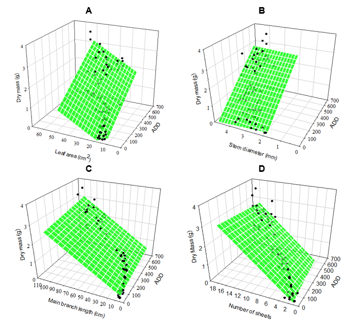
Figure 3 – Graphic illustration of 3D-Plan models adjusted with dependent variable Dry mass and independent variables: A) Accumulated Degree Days and Leaf Area; B) Accumulated Degree Days and Stem Diameter; C) Accumulated Degree Days and Main Branch Length; D) Accumulated Degree Days and Number of Leaves.
It is observed that in both response curves the behavior was linear, that is, the dependent variable dry mass tends to increase with the increase in the independent variables, leaf area, stem diameter, length of the main branch and number of leaves, respectively. These results corroborate the explanations presented in the works of several authors (Reis, 1978, Peixoto, Cruz and Peixoto, 2011; Silva, et al., 2023; Vilas Bôas et al., 2023) whose topics discussed were: Growth analysis plant growth measurement; Quantitative analysis of plant growth – concepts and practice; Adjustment of nonlinear mixed models on blackberry fruit growth; Study of dry matter accumulation in corn hybrids using nonlinear models
CONCLUSIONS
The 3D-flat models whose independent variables were ADD, CPR and DC presented better adjusted coefficients of determination (0.935). While in the 2D models with sigmoid curves, the 4-parameter Sigmoid model was the one that best adjusted the plant growth data with an adjusted R2 of 0.870. In this sense, we can infer that the dry mass of the aerial part of the seedlings has a high positive linear correlation with the ADD. Furthermore, the greatest relative growth followed by stability of the number of leaves and dry mass values was achieved at 346.60 oC ADD in this model, respectively.
The loofah seedlings evaluated in this work had on average: 8.7 leaves per plant, 26.84 cm2 of leaf area per leaf, 3.64 mm in stem diameter and 40.52 cm in length of the main branch and 82.45% water content respectively.
Furthermore, it was possible to conclude that it is extremely important to break the dormancy of loofah seeds well and that the sub-irrigation system effectively controls the attack of leaf-cutter ants. Although, if poorly managed (high water depth) it can contribute to the appearance of leaf chlorosis.
ACKNOWLEDGEMENT
The authors would like to thank the Federal University of Vale do São Francisco (Univasf) for the space, and all the members and collaborators of EngBICS – study group on Biosystems Engineering and Coexistence with the Semiarid and NOA – Center for Studies in Olericulture and Agroecology for their unconditional help in carrying out fieldwork.
BIBLIOGRAPHIC REFERENCES
AZARIAS, E.C.P.; GONZAGA, N.A; MACHADO, L.E.M.; MUNIZ, J.A.; SILVA, E.M. Uso dos modelos Von Bertalanffy e Logístico na descrição do acúmulo de massa seca das plantas daninhas Amaranthus Retroflexus e Amaranthus Hybridus. Revista Foco. Curitiba (PR). v.16.n.7 e2342. p.01-17. 2023b
AZARIAS, E.C.P.; SALVADOR, R.C., SILVA, E.M.; MUNIZ, J;A.; MACHADO, L.E.M. Descrição das curvas de germinação de plantas daninhas em diferentes temperaturas por modelos não lineares. In: Sigmae, Alfenas, v.12, n.3, p. 1-9. 2023a. 67ª Reunião Anual da Região Brasileira da Sociedade Internacional de Biometria (RBras) e 20º Simpósio de Estatística Aplicada `a Experimentação Agronômica (SEAGRO). ISSN: 2317-0840
CALLEGARI-JACQUES, S.M. Bioestatística: princípios e aplicações. Artmed Editora, 2009, 253 páginas
CARMO, V.M.S. Modelos Sigmoidais e Suas Aplicações. 2022. 57 f. TCC (Graduação) – Curso de Engenharia Química, Universidade Estadual Paulista “Júlio de Mesquita Filho”, Araraquara, 2022.
CARVALHO, J.D.V. DOSSIÊ TÉCNICO: cultivo de bucha vegetal. Brasília: Centro de Apoio Ao Desenvolvimento Tecnológico da Universidade de Brasília – Cdt/Unb, 2007. 18 p.
DA SILVA, E.M.; TADEU, M.H.; DA SILVA, E.M.; PIO, R; FERNANDES, T.J; MUNIZ, J.A. Adjustment of mixed nonlinear models on Blackberry fruit growth. Rev. Bras. Frutic., v.45, e-665 DOI: https://dx.doi.org/10.1590/0100-29452023665
FERNANDES, J.G.; DA SILVA, E.M.; GONZAGA, N.A.; AZARIAS, E.C.P.; SILVA, E.M.; FERNANDES, T.J.; MUNIZ, J.A. (2023). Avaliação de modelos não lineares na descrição da curva de crescimento do fruto de pessegueiro “aurora 1”.Revista Foco,16(9), e2993. https://doi.org/10.54751/revistafoco.v16n9-174
GAONA, R.C. Modelagem da composição química do leite através de indicadores metabólicos em vacas leiteiras de alta produção. 2006. 114 f. Tese (Doutorado) – Curso de Veterinária, Universidade Federal do Rio Grande do Sul, Porto Alegre.
GRAPPADELLI, L. C. Application of the expolinear model to define the peak of cytokinesis in apple fruit. Gronn kunnskap, v.9, n. 105B, p.1-3, 2005. IBGE. Instituto Brasileiro de Geografia e Estatística. 2010. http://www.ibge.gov.br/home/estatistica/economia/pam/2010/default_pdf.shtm
GUIMARÃES, I.P.; PEREIRA, F.E.C.B.; DA SILVA, F.G.; DE ARAÚJO, M. D.; SOUZA, P.S.L. Emergência e desenvolvimento de bucha (Luffa Cylindrica Roemer) submetida a diferentes níveis de salinidade. Enciclopédia Biosfera, Centro Científico Conhecer – Goiânia, v.9, N.16; p. 2013
HONORATO, A. C.; PIMENTEL, M. S.; MELO JÚNIOR, J. C. F.; ARAÚJO, E. S. Ajuste do modelo de crescimento expolinear para o feijão-caupi cultivado no Vale do São Francisco. In: CONGRESSO BRASILEIRO DE ENGENHARIA AGRÍCOLA, 43., 2014, Campo Grande. Anais… Campo Grande: Associação Brasileira de Engenharia Agrícola, 2014.
LYRA, G.B.; ZOLNIER, S.; COSTA, L.C.; SEDIYAMA, G.C.; SEDIYAMA, M.A.N. Modelos de crescimento para alface (Lactuca sativa L.) cultivada em sistema hidropônico sob condições de casa-de-vegetação. Revista Brasileira de Agrometeorologia, Santa Maria, v.11, n.1, p.69-77, 2003.
MACHADO, L.E.M.; GONZAGA, N.A.; AZARIAS, E.C.P.; MUNIZ, J.A.; SILVA, E.M. (2023). Ajuste de modelos não lineares para descrever a germinação de sementes de brachiaria brizantha cv. Marandu. Revista Foco, 16(6), e2221. https://doi.org/10.54751/revistafoco.v16n6-052
MAIA, V.R.O.; COSTA FILHO, J.H.; FERREIRA, M.S.; CARVALHO, N.F.O.; SILVA, S.C.A.; DIAS, M.E.M. Caracterização morfoagronômica de acessos de bucha vegetal (Luffa spp.). Acta Iguazu, Cascavel, v. 8, n. 4, p. 132-145, 30 out. 2019.
MAROUELLI, W.A.; DA SILVA, H.R., LOPES, J.F. Circular técnica 116 – Irrigação na cultura da bucha vegetal. Brasília, DF Março, 2013. ISSN 1415-3033
MATOS, A.T. Manual de Análise de Resíduos Sólidos e Águas Residuárias. Viçosa: Ufv, 2015. 149 p.
MELO JÚNIOR, J.C.F; LIMA, A.M.N.; CAVALCANTE, Í.H.L.. Ajuste do modelo expolinear para o crescimento de mudas de mamoeiro cultivadas em Petrolina, PE. In: CONGRESSO BRASILEIRO DE ENGENHARIA AGRÍCOLA – CONBEA, 44., 2015, Petrolina – Pe.CONBEA. São Pedro – Sp, 2015. p. 1-4.
MIOT, H.A. Correlation analysis in clinical and experimental studies. Jornal Vascular Brasileiro, Botucatu, v. 17, n. 4, out-dez. 2018.
MOURA, M.S.B.; SOUZA, L.S.B.; SILVA, T.G.F.; SOARES, J.M.; CARMO, J.F.A.; BRANDÃO, E.O. Modelos de crescimento para o feijão-caupi e o milho, sob sistemas de plantio exclusivo e consorciado, no semiárido brasileiro. Revista Brasileira de Agrometeorologia, v.16, n.3, p.275-284, 2011.
OLIVEIRA. J.L. Potencial energético da gaseificação de resíduos da produção de café e eucalipto. Dissertação de mestrado em Engenharia Agrícola Universidade Federal de Viçosa 2010
PARIKH L, C.S.A., GHOSAL, G.K. A correlation for calculating HHV from proximate analysis of solid fuels. Fuel, V.84, p. 487-494. 2005
PARIKH L, C.S.A.; GHOSAL G.K.. A correlation for calculating elemental composition from proximate analysis of biomass materials. Fuel, V.86, p. 1710-1719. 2007
PEIXOTO, C.P., CRUZ, T.V., PEIXOTO, M.F.S.P. Análise quantitativa do crescimento de plantas: conceitos e prática. Enciclopédia Biosfera, Centro Científico Conhecer – Goiânia, vol.7, N.13; 2011
PRIMAK, T.K.; PRAZERES, J.S.; DA ROSA, J.; BONOME, L.T.S. Tratamentos para quebra de dormência de sementes da bucha vegetal (Luffa Cylindrica). In: Anais do SEPE – Seminário de Ensino Pesquisa e Extensão da UFFS. Vol VII (2017). ISSN 2317-7489
RAMOS, M.G.C.; DA SILVA, E.E.; MELO JUNIOR, J.L.A.; MELO, L.D.F.A. Sementes de bucha vegetal submetidas à bioestimulante. Revista Biotemas, 36 (1), janeiro de 2023
REIS, G.G. Análise de crescimento das plantas – mensuração do crescimento. In: programa cooperativo para el desarrollo de los trópicos americanos. Centro de pesquisa agropecuária do tropico úmido. Curso multinacional de capatación de sistemas integrados de producción agrícola para ia amazónia – IICA trópicos. Belém, Altamira, Pará, Brasil 1978
SA, I. B.;SÁ, I. I. S.;SILVA, A. de S.;SILVA, D. F. da. Caracterização ambiental do Vale do Submédio São Francisco. In: LIMA, M. A. C. de; SA, I. B.; KIILL, L. H. P.; ARAUJO, J. L. P.; BORGES, R. M. E.; LIMA NETO, F. P.; SOARES, J. M.; LEAO, P. C. de S.; SILVA, P. C. G. da; CORREIA, R. C.; SILVA, A. de S.; SÁ, I. I. S.; SILVA, D. F. da Subsídios técnicos para a indicação geográfica de procedência do Vale do Submédio São Francisco: uva de mesa e manga. Petrolina: Embrapa Semiárido, 2009. p. 8-15. (Embrapa Semiárido. Documentos, 222).
SILVA, É.M., TADEU, M.H., SILVA, E.M., PIO, R., FERNANDES, T.J., MUNIZ, J.A. Adjustment of mixed nonlinear models on Blackberry fruit growth. Rev. Bras. Frutic., v.45, e-665 2023 DOI: https://dx.doi.org/10.1590/0100-29452023665
SIQUEIRA, R.G.; SANTOS, R.H.S.; MARTINEZ, H.E.P.; CECON, P.R. Crescimento, produção e acúmulo de nutrientes em Luffa Cylindrica M. Roem. Rev. Ceres, Viçosa, v. 56, n.5, p. 685-696, set/out, 2009
SOUZA, L.S.B.; MOURA, M.S.B.; SILVA, T.G.F.; SOARES, J.M.; SANTOS, W.S. Ajuste do modelo de crescimento expolinear para o feijão caupi no semiárido brasileiro. In: CONGRESSO BRASILEIRO DE AGROMETEOROLOGIA, 15., 2007, Aracaju. p. 1-5.
VADERA, H.R., PANDYA, J.B., MEHTA, S.K. Developmental changes in seedlings of Luffa Cylindrica M. Roem. and Momordica Charantia L. due to the seed germination treatments. Asian Journal of Plant and Soil Sciences. 6(2): 23-36, 2021
VELOSO, R.C.; WINKELSTROTER, L.K.; SILVA, M.T.P.; PIRES, A.V.; TORRES FILHO, R.A.; PINHEIRO, S.R.F.; COSTA L.S.; AMARAL, J.M. Seleção e classificação multivariada de modelos não lineares para frangos de corte. Arq. Bras. Med. Vet. Zootec., v.68, n.1, p.191-200, 2016
VILAR, D. A Importância da Água para as Plantas. 2021. Disponível em: https://agriconline.com.br/portal/artigo/a-importancia-da-agua-para-as-plantas/#:~:text=A%20%C3%A1gua%20atua%2C%20tamb%C3%A9m%2C%20comoTAIZ%3B%20Z%20EIGER%2C%202002. Acessado em 12/04/2024
VILAS BÔAS, I.A.; FERNANDES, F.A.; FERNANDES, T.J.; MUNIZ, J.A. Study of dry matter accumulation in maize hybrids using nonlinear models. Pesquisa Agropecuária Brasileira, v.58, e03077, 2023. DOI: https://doi.org/10.1590/S1678-3921.pab2023.v58.03077
1Doutor em engenharia agrícola pela Universidade Federal de Viçosa – UFV. Docente efetivo da Universidade Federal do Vale do São Francisco – Univasf BR 407, km119, Projeto de Irrigação Senador Nilo Coelho, Lote 543, Petrolina – PE – Brasil. neiton.machado@univasf.edu.brhttps://orcid.org/0000-0001-6049-2279
2Bacharel em engenharia agronômica pela Universidade Federal do Vale do São Francisco – Univasf BR 407, km119, Projeto de Irrigação Senador Nilo Coelho, Lote 543, Petrolina – PE – Brasil. feliperodrigues9526@gmail.com https://orcid.org/0009-0000-7606-2177
3Doutora em engenharia agrícola pela Universidade Federal de Campina Grande – UFCG. Docente efetivo da Universidade Federal do Vale do São Francisco – Univasf BR 407, km119, Projeto de Irrigação Senador Nilo Coelho, Lote 543, Petrolina – PE – Brasil. karla.smsousa@univasf.edu.br https://orcid.org/0000-0001-5000-0330
4Doutor em biometria e estatística aplicada pela Universidade Federal Rural de Pernambuco – UFPE Docente efetivo da Universidade Federal do Vale do São Francisco – Univasf BR 407, km119, Projeto de Irrigação Senador Nilo Coelho, Lote 543, Petrolina – PE – Brasil. adriano.victor@univasf.edu.br https://orcid.org/0000-0002-5923-3015
5Doutor em engenharia agrícola pela Universidade Federal de Viçosa – UFV. Docente efetivo da Universidade Federal do Vale do São Francisco – Univasf BR 407, km119, Projeto de Irrigação Senador Nilo Coelho, Lote 543, Petrolina – PE – Brasil. daniel.mariano@univasf.edu.br https://orcid.org/0000-0002-6174-1190
6Doutor em engenharia agrícola pela Universidade Federal de Viçosa – UFV. Docente efetivo da Universidade Federal do Vale do São Francisco – Univasf BR 407, km119, Projeto de Irrigação Senador Nilo Coelho, Lote 543, Petrolina – PE – Brasil. julio.melo@univasf.edu.br https://orcid.org/0000-0003-3843-9724