REGISTRO DOI: 10.5281/zenodo.10849903
Raimundo N. C. Souza1
André L. A. Mesquita2
Heliton Ribeiro Tavares3
The population growth model is described by a differential equation with an exponential function as its solution. Depending on the sign of the constant, the exponential function either grows or decays. In SOUZA (2019), the probability of an avalanche extending to a certain level is, by hypothesis, considered exponential.Based on that work, we developed this one to prove the hypothesis that says that the probability of avalanche growth follows an exponential decay model. Two approaches were employed to achieve this objective. The first involved a mathematical demonstration, while the second utilized statistical methods such as exponential regression and hypothesis testing.
1. Introduction
The population growth model describes how a population changes over time. There are two main models of population growth: exponential population growth and logistic population growth, [14].
In theory, any type of organism could take over the Earth through reproduction alone. For example, imagine that we initially had a single pair of rabbits, one male and one female. If these rabbits and their offspring reproduced at maximum speed (“like rabbits”) for 7 years, without any deaths, we would have enough rabbits to cover the entire state of Rhode Island,[19].
Population dynamics deals with variations, in time and space, of population densities and sizes. Its study aims to better understand the variation in the number of individuals in a given population and also the factors that influence such variations. To do this, it is necessary to know the rates at which losses and gains of individuals occur and to identify the processes that regulate population variation. The interest in this study is not just theoretical, being important for pest control, animal husbandry, etc. [10]
Population ecologists use a variety of mathematical methods to model population dynamics (how populations change size and composition over time). Some of these models represent growth without environmental constraints, while others include “ceilings” determined by limiting resources. Mathematical population models can be used to precisely describe the changes occurring in a population and, importantly, predict future changes. [19]
Don’t be confused by the word model. In mathematics, we often use the terms function, equation, and model interchangeably, even though each has its own formal definition. The term model is typically used to indicate that the equation or function approximates a realworld situation, [7].
Exponential population growth does not take into account limiting factors, such as finite resources, that is, growth is unlimited. The logistic population growth model considers an upper limit (K) for population growth due to resource availability. Imagine the case of a rumor that spreads within a community, in this case, there will come a time when everyone in the community will be aware of the rumor so there will be nowhere else for it to be spread,thus reaching its ceiling. Initially, growth is exponential, but decreases as the population approaches K. [19]
MSC2020 subject classifications: Primary 92-10, 93Exx ; secondary 60-11, 62-04 ; tertiary 76-05, 76-10 .
Keywords and phrases: Population growth model, Probability, Avalanche.
Stones, snow, mud, grains and even some ores can move in large quantities, very quickly and with unexpected results. Natural phenomena with these characteristics are considered avalanches. There are also avalanches related to the displacement of animals or humans. These occur when a large number of individuals move quickly from one place to another. Avalanches can happen in a simple pile of sand, where movement of the surface layers of the pile of sand can set in due to small disturbances such as adding more grains or tilting the pile. These disturbances can cause avalanches, which are grains sliding on the surface of a granular medium caused by instabilities. Small disturbances can be amplified, giving rise to large mass displacements [23].
The main characteristic of an avalanche is the rapid growth of a number of elements interacting with others, [4]. Avalanches usually occur suddenly and quickly. Where a small disturbance evolves quickly and reaches great dispersion within the environment.
Although it is reasonable to deduce that this rapid increase in avalanche size is due to exponential growth, there is no specific concept of exponential growth applied directly to avalanches in the same way that the exponential model is used to describe population growth. This fact justifies the development of this study.
2. Population growth models.
Population or demographic growth: is the population growth rate [N(t)] calculated from the sum of natural growth and migratory growth, excluding those individuals who ceased to exist and those who changed regions.

It is essential to understand that triggering factors, unstable conditions and safety practices when dealing with or living in areas susceptible to avalanches can change the way avalanche growth occurs, i.e., treating the avalanche as a population, population growth represents the variation in the size of the avalanche.
2.1. The exponential population growth model.
The exponential population growth model describes a constant increase in population over time without taking into account limiting factors. It is the simplest population growth model and can be defined through an exponential growth function, where the population increase responds to a fixed growth rate, not correlated with the size of the population in question, where N is equal to the population and r the constant rate of increase. For example, a cattle herd in which the population grows by artificial insemination and the producer performs a fixed number of this procedure each year [14]. In exponential growth, the population growth rate increases over time in proportion to the size of the population. The central concept of exponential growth is that the rate of population growth — the number of organisms added in each generation — increases as the population gets larger [19].
To understand the different models that are used to represent population dynamics, let’s start by looking at the general equation for population growth rate (change in the number of individuals in a population over time). We can give a more complex interpretation to Equation 1, imagining that both the number of births and the number of deaths are proportional to the total number of individuals that populate the population at that moment in time. So, if α and β are real numbers, the number of births will be (α.N) and the number of deaths will be (β.N). Assuming there is no movement of individuals into or out of the population, the growth rate is only a function of birth and death rates, thus [17]:
(2) ![]()
In this context, the number of individuals entering and leaving the population through immigration are considered null, therefore resulting in a restriction of the model or condition of existence. Exponential population growth is defined by the following equation:
(3) 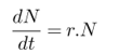
In Equation 3, dN/dt represents the population growth rate at a given time t, N is the population size, t is the time, and r is the per capita growth rate, that is, how quickly a population grows per individual already present in the population [19].
The exponential population growth model was described by Malthus in 1798. Its dynamics arise from cumulative processes (positive or reinforcing feedback). These processes occur when the net variation of the system is proportional to its current state, reinforcing the existing trend. In this model, a population grows according to the constant birth rate r.
Equation 3 is quite general, and we can derive it into more specific forms to describe two different types of growth models: exponential and logistic. When the per capita growth rate (r) assumes the same positive value, regardless of population size, then we have exponential growth. When the per capita growth rate (r) decreases as the population increases towards its maximum limit, then we have logistic growth [20].
When population size, N, is projected over time, a J-shaped growth curve forms. Figure 1.
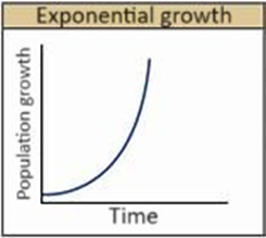
FIG 1. Exponential population growth curve. Image credit: “Environmental limits to population growth: Figure 1,” by OpenStax College, Biology, CC BY 4.0.
The general formula for exponential population growth is given by the Equation 4 which is obtained by solving the Differential Equation in 3, and which gives the model its name.
(4) ![]()
N(t) is the population size at time t. N0 is the initial population size. r is the per capita growth rate. t is time in appropriate units. e is the base of the natural logarithm, approximately 2.71828. If r > 0, then N(t) is an exponentially increasing function of t, which means that the population grows exponentially over time. If r < 0, then N(t) is an exponentially decreasing function of t, which means that the population decreases exponentially with time.
The exponential model assumes unlimited population growth over time, meaning there are no limiting factors such as finite resources or competition, or in the case of the avalanche, infinite material. The growth curve is a positive exponential, resulting in a curve that becomes increasingly steeper as time progresses, as in Figure 1. The model does not take into account environmental constraints that could limit population growth, such as food availability, space, predators or disease. The exponential growth model is often used to describe population growth in early stages, before limiting factors become significant [7].
In reality, all ecosystems have ecological limits that eventually affect population growth, making the exponential model unsuitable for describing long-term population growth. Although the exponential model is a simplification, it is useful in situations where population growth is rapid and limiting factors have not yet come into play [14].
2.2. The logistic population growth model.
Belgian mathematician Pierre F. Verhurst proposed a model in 1837 that assumes that a population can grow up to a maximum limit, after which it tends to stabilize. The model proposed by Verhurst meets a condition in which the effective growth rate of a population varies over time. This model is an alternative to the exponential growth model in which the growth rate is constant and there is no limitation on the growth of population size, [13].
Exponential growth can happen over a period of time if there are few individuals and many resources. But when the number of individuals grows enough, resources begin to run out, slowing the growth rate. Under the conditions of the continuous time model, the growth flow instantly adjusts to slow population growth when the population, N, approaches the carrying capacity, k, of the surrounding environment. Therefore, it is difficult for a population to exceed this support capacity. Any disturbance that causes growth above this threshold, for example, the instantaneous entry of new individuals into the population, is absorbed by a negative feedback mechanism that nullifies the flow of growth and allows the flow of deaths to quickly restore the population to level k .
We can mathematically model logistical growth, modifying our exponential growth equation 3, using a r (per capita growth rate) that depends on the size of the population (N) and its proximity to the load capacity (K). Assuming that the population has a base growth rate rmax when it is very small, we can write the following equation [13]:
(5) ![]()
Let’s analyze this equation to see why it makes sense. At any point in population growth, the expression (K – N) tells us how many individuals can still be added to the population before it reaches its carrying capacity. (K – N)/K is the fraction of the carrying capacity that has not yet been “used”. The more carrying capacity is consumed, the more the (K – N)/K term will reduce the growth rate. When the population is very small, N is very small compared to K. The term (K – N)/K becomes approximately (K/K), or 1, returning to an exponential equation. This fits into our graph in Figure 2, where the population grows almost exponentially at the beginning, but increasingly stabilizes as it approaches K [14].
Logistic growth, sometimes called sigmoidal, involves exponential population growth, as we have already mentioned, followed by a steady reduction in population growth until the population size stabilizes, taking on an S-shaped curve, hence the name sigmoidal [19](Figure 2).
An example of logistical growth is the case of yeast, [1]. A microscopic fungus used to make bread and alcoholic beverages that can produce a classic S-shaped curve when grown in a test tube. Yeast growth stabilizes when the population reaches the limit of available nutrients in the flask. When monitoring the fungal population for some time, it would probably collapse, since the test tube is a closed system, meaning energy sources would run out and waste could reach toxic levels.
The logistic differential equation is a separable differential equation, so when solving it we arrive at the solution:
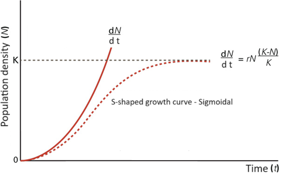
FIG 2. Exponential increase (solid line) and sigmoidal increase (dashed line) of population density (N) over time. Source: Adapted from Begon[26] .
(6) 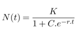
Where ![]() is the initial number of the population. In the case of a pandemic, N0= 1, as every epidemic starts from an individual [26]. This is also the case with the beginning of an avalanche as described in [23]. It is common for real populations to continually oscillate (backwards or forwards) around carrying capacity, rather than forming a perfect straight line.
is the initial number of the population. In the case of a pandemic, N0= 1, as every epidemic starts from an individual [26]. This is also the case with the beginning of an avalanche as described in [23]. It is common for real populations to continually oscillate (backwards or forwards) around carrying capacity, rather than forming a perfect straight line.
3. The growth of the avalanche
In the model proposed in [23], the avalanche is idealized as a surface network of grains where only surface grains participate in the event. The grains are called avalanche sites and do not depend on a conventional form of energy to interact with each other, but rather on a probability of activation. Once activated, the site can make its neighbors active. Specifically in this model, there is a barrier, a randomness that needs to be overcome so that the site can activate and transmit “energy” to neighboring sites. Thus, making the avalanche a process of transmitting activity from site to site. If the probability of activation of the site is low, and the site does not activate, then the process of transmitting activity from that site ends. The sites are configured with a certain probability of receiving activity, in this way the active site transmits activity to its neighbors, while the inactive site does not.
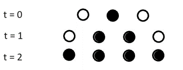
FIG 3. Transmission of activity between avalanche sites. Source: Adapted from [22].
Consider that this probability of activation is maximum, so if there is an active site in the neighborhood, all the others become active too. However, we will direct the order of activation, as we want the behavior of an avalanche that moves in an oriented direction as in Figure 3.
Looking at Figure 3, the white balls are inactive, the black ones are active and increase in quantity as t grows. Let’s define two quantities: The number of active sites at time t is denoted by N(t), while the quantity “avalanche size” is defined by a variable T. It is possible to conclude that N(t), the number of sites active at time t, is given by the equation:
(7) N(t)=2t
Clearly, Equation 7 is an exponential with base 2, N0=1 and r =1, while t – which would be time, in this model, it represents the distance of the layer of points in relation to the site that gave rise to the avalanche , that is, size T.
(8) T ∼ t
With Equation 8, we do not mean that time and space are equal, but rather that the distance from the origin to layer t are counted on the same scale. That is, if t = 1 then T = 1 and vice versa. Thus, we can infer that the population growth of active avalanche sites is governed by an exponential population growth model. In this scenario, the avalanche would extend indefinitely.
However, the maximum activation probability hypothesis does not apply in reality. There will be at some time t, among the N(t), at least one inactive site X. This affects the precision of equation 7, in the sense that the real N(t) is always smaller than the theoretical N(t) [given by Equation 7]. Briefly, for real avalanche events, calculating N(t) using Equation 7 would only be an estimate of the true value.
Take as an example the law of exponential decay of radioactive nuclei. With R being the probability of radiation emission per second and assuming that N nuclei have not decayed at time t. After the interval dt, a dN = – NR dt number of nuclei will decay. Since R is the probability that a particular nucleus decays in one second, Rdt is the probability that any of the system’s nuclei decay in that time interval, described by an exponential-type power law. We can demonstrate that the time interval necessary for the number of nuclei, which have not yet decayed, decreases by a factor equal to two, [21]. If instead of a nucleus there were initially a total of N0 identical nuclei, the number N of nuclei without undergoing decay after time t would be:
(9) N(t)= N0 . e−R.t
Take a handful of rice and place the grains, one by one, on a table, to form a pile. The pile won’t grow forever. Adding one more grain, sooner or later, will cause an avalanche. But this grain will be special only because it fell in the right place at the right time. The addition of a grain could have had no effect, or else precipitated a small avalanche. But it could have brought down the entire structure, [8]. We can predict the frequency of avalanches, but not when they will occur or their size. It is not surprising that larger avalanches will occur less frequently than smaller ones. What is surprising is that we again have a power law: by doubling the size of the grain avalanche, it becomes twice as frequent, [2]. The apparent complexity of a pile of grains collapses into the simplicity and hidden order of a power law,[10].
The concept of survival probability – P(N(t)≥1) – is connected to the theoretical perspective of a complex system generating events over time, [15]. A complex system at criticality generates that are referred to as crucial events. [12], mentions that the probability of survival has the form P(N(t)≥1)= t−β. On the other hand,[18] indicates that this probability can e generalized by P(N(t)≥1)= αt−β. These literatures diverge in part when the intention is to give a formulation for P(N(t)≥1). The consensus between both is that the probability of survival is given by a power function. However, we are convinced that this probability can be represented by a decreasing exponential function, that is, it has exponential decay, which would make the probability function come from a population growth model.
By carrying out an experiment that simulates real avalanches, M times, and keeping the size (T) of each avalanche, we obtain a diverse amount of values that represent the size of the avalanches. Of these M, only m avalanches have size T. It is possible to estimate the probability of having an avalanche of size T, assuming that this probability can be represented by the simple relative frequency.
(10) ![]()
Another important probability is the probability of an active site existing at time t. Let’s imagine that all sites at time t-1 are active, so, at time t, the probability of N(t)= n is given by:
(11) ![]()
Where ![]() is the combination of 2t sites that can be activated at time t and n ≤2t. For example, if t =2 and we want to know the probability of N(t)=1 then P(N(t =2)=1)= 0.25. We can calculate the probability of there being at least 1 active site at time t, with the hypothesis that at t −1 all sites are active:
is the combination of 2t sites that can be activated at time t and n ≤2t. For example, if t =2 and we want to know the probability of N(t)=1 then P(N(t =2)=1)= 0.25. We can calculate the probability of there being at least 1 active site at time t, with the hypothesis that at t −1 all sites are active:
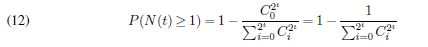
Knowing that the sum of the combinations is equal to 22t, we can rewrite Equation 12:
(13) P(N(t)≥1)=1−2−2t
4. Probability and decay.
A single differential equation can serve as a mathematical model for studying different phenomena. The two problems mentioned above, radioactive decay and avalanche growth, use the same mathematical model, differing only in the proportionality constant in which one is negative and the other is positive. This same model can be used to study the growth of capital at continuously compounded interest, the half-life of a drug, etc. [25].
In mathematics, exponential decay occurs when an original quantity is reduced by a consistent rate (or percentage of the total) over a period of time. A real purpose of this concept is to use the exponential decay function to make predictions about market trends and expectations of imminent losses. Basically, the exponential decay formula can be used in any situation where a quantity of something decreases by the same percentage with each iteration of a measurable unit of time, [14].
In a radioactive substance, each atom has a certain probability, per unit of time, of transforming into a lighter atom, emitting nuclear radiation in the process. If R represents this probability, the average number of atoms that transmute, per unit of time, is RN, where N is the number of atoms existing at each instant. The number of atoms transmuted per unit of time is also equal to minus the temporal derivative of the N function, [27]. R, the probability, is a constant, called the decay constant. The greater the decay constant R, the faster the mass of the substance decreases.
Now that we understand that both population growth and exponential decay share the same mathematical model, we can explore the exponential equation that describes the probability of survival in an avalanche.
The relationship between probability and exponential decay is generally associated with stochastic processes in which the probability of an event occurring decreases exponentially over time [9]. A classic example is the concept of half-life in radioactive decay processes [11]. The probability of a radioactive atom decaying within a given time interval follows an exponential distribution. The formula for the probability P(t) of a radioactive atom not having decayed after time t is given by the exponential decay function:
(14) P(t)= e−λt
Where λ is the decay constant (related to the decay rate), t is the time. Thus, the probability of survival, that is, the probability that decay has not occurred by time t, decreases exponentially with time.
In more general contexts, exponential decay can be used to model processes in which the probability of an event occurring decreases over time at a constant rate. The probability of the event not having occurred by a certain point in time is described by the exponential function. This type of modeling is common in statistics, queuing theory, probability theory and other fields in which randomness and time play important roles, [24].
The random variable for the exponential distribution is continuous and generally measures the passage of time, although it can be used in other applications. Typical questions might be: what is the probability that some event will occur in the next t hours or days, or what is the probability that some event will occur between t1 hours and t2 hours, or what is the probability that the event will take more than t1 hours to run. The probability density function (pdf) is given by [16]:
(15) ![]()
An alternative form of the exponential distribution formula recognizes what is often called the decay factor. The decay factor simply measures how quickly the probability of an event decreases as the random variable T increases. When notation using the decay parameter m = 1/µ is used, the probability density function is presented as:
(16) f(t)= m e−mt
To calculate probabilities for specific probability density functions, the cumulative density function (cdf) is used. The cumulative density function is simply the integral of the pdf:

The connection between probabilities and population growth models is notable, see Equation 13. When exploring the growth dynamics of a population, we can apply probabilistic concepts to better understand the events that influence this growth over time. In many cases, probabilities are intrinsically linked to patterns of variation in the population. For example, when considering the exponential growth model in population biology, the probability of a specific individual contributing to the next generation can be associated with its reproduction rate. Similarly, in the context of exponential decay, the probability of an event occurring or not occurring over time can be expressed by an exponential function.
This relationship becomes even more evident in scenarios where random events, such as activation (birth) and inactivation (death), play crucial roles in avalanche (population) growth.
5. Building an exponential growth model from data.
There are many situations that can be modeled by exponential functions, such as investment growth, radioactive decay, changes in atmospheric pressure and temperatures of a cooling object, [10]. The way the data grows or shrinks helps us determine whether it is best modeled by an exponential equation. Knowing the behavior of exponential functions in general allows us to recognize when to use exponential regression to represent data from those events that have exponential growth or decay.
In the previous parts of this work, we had two different approaches to dealing with exponential growth models. In some cases we were given an explicit function and in others algebraic methods were used to determine the equation that precisely fits the mathematical model.
However, in this section we explore a modeling technique known as regression analysis. This method is employed to find a curve that best fits data collected through real-world observations. Rather than starting with a specific function or points, regression analysis allows us to identify patterns in data and develop an equation that generally represents the behavior of that observed data [6].
This approach is particularly useful when dealing with complex data sets from practical observations, allowing us to create models that are more flexible and adaptable to the nuances of the real world. Furthermore, it will be definitive proof that the avalanche survival probability curves are exponential functions [23].
With regression analysis, we don’t expect every point to be perfectly on the curve. The idea is to find a model that best fits the data. We then use the model to make predictions about future events.
Exponential regression is used to model situations where growth starts slowly and then accelerates rapidly without limit, or where decay starts quickly and then slows to get closer and closer to zero [3]. When performing regression analysis, we use the most commonly used form [6]:
(18) Y = a.bX
Where a > 0, b must be greater than zero and different from 1. If b > 1, the function models exponential growth. As X increases, the model outputs increase slowly at first, but then increase more and more quickly, without limit. If 0 < b < 1, the function models exponential decay. As X increases, the model outputs decrease rapidly at first and then level off to become asymptotic about the X axis.
5.1. Exponential Regression Method.
Exponential regression is a statistical method used to fit an exponential curve to a set of data. The objective is to find the exponential equation that best fits the observed data. Analyze the data and determine if there is an underlying exponential trend. In an exponential regression, data is expected to increase or decrease exponentially. Exponential regression follows the general model P = abT , where a and b are constants and T is the independent variable.
If necessary, transform the data to make it linearly related. A common way is to use the natural logarithm (ln) of the values, which converts the exponential equation into a linear form [6]:
(19) ln(P)= ln(a)+ T ln(b)
Exponential regression is fitted using the natural logarithm, after logarithmic transformation of the data. The model coefficients are then exponentiated to obtain the parameters of the original exponential equation. Then the straight line fitting technique (linear regression) is applied to the transformed data. This can be done using statistical tools or data analysis software. As part of the results, it is necessary to calculate a number known as the correlation coefficient, labeled by the variable R-squared.
In general, a model fits the data well if the differences between the observed values and the model’s predicted values are small and unbiased. Before looking at the statistical measures of the goodness-of-fit test, you should check the residual plots. Residual plots can reveal unwanted patterns in the residuals, which indicate biased results more effectively than numbers. When the residual plots are accepted, you can trust the numerical results and verify the goodness-of-fit test statistics [3].
The R-squared is a statistical measure of how close the data is to the fitted regression line. It is also known as the coefficient of determination or the coefficient of multiple determination for multiple regression. The definition of R-squared is quite simple: it is the percentage of variation in the response variable that is explained by a linear model. Or: R-squared = Explained variation/Total variation [5].
R-squared is calculated using the conventional formula for the coefficient of determination, comparing the variation explained by the model with the total variation in the data. R-squared is always between 0 and 100%. R−squared =0% indicates that the model does not explain any of the variability of the response data around its mean. 100% indicates that the model explains all the variability of the response data around its mean. In general, the higher the R-squared, the better the model fits your data [6].
5.2. Exponential Regression applied to avalanche data.
Applying exponential regression to avalanche data will play a crucial role in understanding and predicting these complex natural events. When analyzing a dataset on real laboratory avalanches, we can employ exponential regression to model the probability of these events occurring [22].
Exponential regression is particularly useful when examining the temporal evolution of avalanches, allowing the identification of patterns of growth and decay associated with different conditions. For example, the growth rate over time can be modeled using exponential regression to predict which layer it will reach and what the critical probability is, and the factors that increase the probability of triggering the avalanche.
Furthermore, applying exponential regression to avalanche data can contribute to the development of more accurate early warning systems. Mathematical models based on exponential regression can be integrated with real-time monitoring technologies, allowing continuous assessment of avalanche risks in prone regions. This approach offers a valuable tool for disaster management and the protection of communities vulnerable to these natural events, by enabling a better understanding of the temporal dynamics of avalanches and their potential consequences.
However, the main focus lies on demonstrating that the avalanche probability curve exhibits behavior compatible with an exponential curve. By collecting and analyzing data related to avalanche events over time, the application of exponential regression allows you tomodel the probability of occurrence of these events in a systematic way. Let’s analyze the behavior of 10 thousand real avalanches, carried out as described in [23]. T size data is shown in table 1:
TABLE 1
Size data from 10 thousand real avalanches created by the methodology described in SOUZA, 2019.
Size Frequency Relat. Freq. Abs. Freq. 1-10 7736 0,7736 0,7736 11-20 1545 0,1545 0,9281 21-30 488 0,0488 0,9769 31-40 145 0,0145 0,9914 41-50 58 0,0058 0,9972 51-60 11 0,0011 0,9983 61-70 9 0,0009 0,9992 71-80 4 0,0004 0,9996 81-90 1 0,0001 0,9997 91-100 3 0,0003 1
Let’s create an exponential regression using this data in Rstudio software. However, first let’s visualize the data by creating a quick scatterplot to visualize the relationship between P (Relative Frequency) and T (Size). Figure 4.
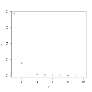
FIG 4. Scatterplot of P (relative frequency) versus T (Size) of data from 10 thousand real avalanches. Plotted in Rstudio software.
Note that in real-world situations, data may require more sophisticated analysis, and it is important to carefully consider the interpretation of results. In the graph, we can see that there is a clear pattern of exponential decay between the two variables. Therefore, it seems sensible to fit an exponential regression equation to describe the relationship between the variables.
We will use the lm() function to fit an exponential regression model, using the natural logarithm of P as the response variable and T as the predictor variable. The code that performs this task is in Annex I. The regression graph for this data is shown in Figure 5.
The exponential regression coefficients are a = 0.8640853 (called the intercept) and b = 0.3882302 (called the time-associated coefficient) and R − squared = 0.9427598 = 94.27598%.
Additionally, in Rstudio it is also possible to perform a hypothesis test, in which the null hypothesis is that the regression does not fit the data. This test is performed using the Rstudio routine. In the Table 2, this routine and the result of the hypothesis test are exposed.
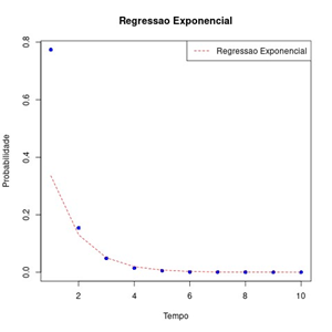
FIG 5. Exponential regression graph for data from 10 thousand avalanches. Plotted in Rstudio software.
TABLE 2
Application of the Rstudio exponential regression routine to the data and the result of the hypothesis test.
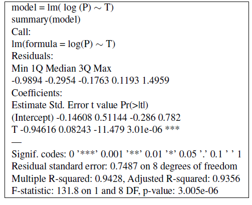
The linear equation can be obtained in R using the lm() function, which is used to calculate simple linear regression. And it can only be applied in this context due to the transformation Y into logarithm of P that linearizes the exponential equation.
Regarding hypothesis testing: When performing a hypothesis test in exponential regression analysis, the conclusion that the null hypothesis should be rejected generally suggests that there is significant statistical evidence that the relationship between the variables is not explained by a relationship linear, but rather by an exponential relationship. Rejecting the null hypothesis implies that the data provides sufficient evidence to suggest that the relationship between the variables is better modeled by an exponential curve than by a straight line. As the p-value is equal to 3.005×10⁻⁶ which is significantly less than the usual significance level of 0.05, then it can be concluded that there is sufficient statistical evidence to reject the null hypothesis and conclude that the relationship between the variables is best explained by an exponential relationship.
6. Conclusion
Therefore, we conclude that avalanche growth probabilities not only can, but often should, be incorporated into population growth models. In doing so, we gain a more comprehensive and realistic understanding of the processes that drive the growth of avalanches over time, offering a new interpretation for modeling these events. This interconnection between probability and population growth highlights the importance of a holistic approach when studying and modeling dynamic phenomena in nature.
By highlighting the exponential nature of the probability of avalanches, the results of the analysis reinforce the importance of mathematical strategies in approaching complex systems. Understanding the underlying dynamics through exponential regression allows for a more accurate approach to evaluating these events in susceptible areas.
These results corroborate a new interpretation of the probability function, because as mentioned it was believed that the probability function is a power law but as shown, it is classified as an exponential function that comes from an exponential decrease model. This is in line with the modeling carried out by [23], where the accumulated probability was given as a joint exponential.
REFERENCES
- AE, O. D. A. E. (2023). MODELOS DE FUNÇÕES DE CRESCIMENTO. MATEMÁTICA 37.
- BAK, P., TANG, C. and WIESENFELD, K. (1987). Self-organized criticality: an explanation of 1/f noise, 1987. Phys. Rev. Lett 59 381.
- BEALE, C. M., LENNON, J. J., YEARSLEY, J. M., BREWER, M. J. and ELSTON, D. A. (2010). Regression analysis of spatial data. Ecology letters 13 246–264.
- BROADBENT, S. R. and HAMMERSLEY, J. M. (1957). Percolation processes: I. Crystals and mazes. In Mathematical Proceedings of the Cambridge Philosophical Society 629–641. Cambridge University Press.
- CAMERON, A. C. and WINDMEIJER, F. A. (1997). An R-squared measure of goodness of fit for some common nonlinear regression models. Journal of econometrics 77 329–342.
- CAVALCANTI, A. B. (2009). Aperfeiçoamento de métodos estatısticos em modelos de regressao da famılia exponencial, PhD thesis, Tese de doutorado. Sao Paulo: IME–USP.
- DE MENEZES, M. L., STRÖHER, A. P., PEREIRA, N. C. and DE BARROS, S. T. D. (2013). Análise da cinética e ajustes de modelos matemáticos aos dados de secagem do bagaço do maracujá-amarelo. Engevista 15 176–186.
- FRETTE, V. (1980). Avalanche Dynamics in a Pile of Rice. Nature 40 379–384.
- GALLAGER, R. G. (2013). Stochastic processes: theory for applications. Cambridge University Press.
- GLERIA, I., MATSUSHITA, R. and SILVA, S. D. (2004). Sistemas complexos, criticalidade e leis de potência. Revista Brasileira de Ensino de Física 26 99–108.
- GROCH, M. W. (1998). Radioactive decay. Radiographics 18 1247–1256.
- HINRICHSEN, H., JIMÉNEZ-DALMARONI, A., ROZOV, Y. and DOMANY, E. (2000). Flowing sand—a possible physical realization of Directed Percolation. Journal of Statistical Physics 98 1149–1168.
- KINT, J., CONSTALES, D. and VANDERBAUWHEDE, A. (2006). Pierre-François Verhulst’s final triumph.The logistic map and the route to chaos: from the beginnings to modern applications 13–28.
- LEDWITH, J. (2020). Decadência exponencial na vida real – real life use exponential function. Greelane.
- LUKOSEVICIUS, A. P., MARCHISOTTI, G. G. and SOARES, C. A. P. (2016). Panorama da complexidade:principais correntes, definições e constructos. Sistemas & Gestão 11 455–465.
- MAGALHÃES, M. N. (2006). Probabilidade e variáveis aleatórias. Edusp.
- MALTHUS, T. R. (1986). An essay on the principle of population (1798). The Works of Thomas Robert Malthus, London, Pickering & Chatto Publishers 1 1–139.
- MEC-MCT, P. C., DE OLIVEIRA, S. R. et al. (2010). Avalanches.
- MIRAUX, L. (2022). Environmental limits to the space sector’s growth. Science of The Total Environment 806 150862.
- NÁPOLES, S. (2018). O crescimento exponencial de populações: Euler ou Malthus? Revista de Ciência Elementar 6.
- SALINAS, S. R. (1999). Introdução à física estatística. Edusp.
- SOUZA, R., TAVARES, H. and MESQUITA, A. L. A. (2023). MODELO PARA AVALANCHE SOB ENFOQUE DA TEORIA DA PERCOLAÇÃO. RECIMA21-Revista Científica Multidisciplinar-ISSN 2675-6218 4 e4114430–e4114430.
- SOUZA, R. N. C. D. et al. (2019). Avalanche como rede de percolação não homogênea, PhD thesis, Universidade Federal do Pará.
- TAVARES, H. R., SOUZA, R., MADRUGA, M. and FARIAS, V. (2015). Densidade Crítica no Modelo de Percolação em Rede de Bethe Não-Homogênea. TEMA (São Carlos) 16 173–182.
- TAVONI, R. (2013). Os modelos de crescimento populacional de Malthus e Verhulst: uma motivação para o ensino de logaritmos e exponenciais.
- TOWNSEND, C. R., BEGON, M. and HARPER, J. L. (2009). Fundamentos em ecologia. Artmed Editora. [27] VILLATE, J. E. (2001). Equações diferenciais e equações de diferenças.
1Universidade Federal do Pará,
raimundosouza@ufpa.br
2Universidade Federal do Pará,
andream@ufpa.br
3Universidade Federal do Pará
heliton@ufpa.br