REGISTRO DOI: 10.5281/zenodo.7878789
Jessica A. Sciammarelli1
1. Problem Statement and literature review
1.1 Introduction
The brain is the most complex part of the human body that controls memory, emotions, touch, motor, thought, skills, vision, breathing, temperature and every process related to regulating the human body. Usually, the brain tumour can be classified as malignant or benign, and it can spread to other regions as sometimes not. (MRI) Magnetic Resonance Imaging is the most common exam to identify the tumours, and later the resection surgery as a decision that has to be made from neurosurgeon. The specialized doctor has to mark the tumour region precisely and a manual method can be high time-consuming work for a doctor.
Deep Learning has improved and demonstrated efficiency in many tasks, in special, the (CNN)Convolutional Neural Networks has achieved the state-of-the-art in performing medical image segmentation tasks. Nowadays it is possible to segment tumours in any kind of shape, size and contrast through machine learning models, using MRI images. 3 D U-Net architecture was selected because it is specialized for brain tumours segmentations and has been successfully utilized for this type of tasks in the research field.
Generally, U-Net architectures utilize fully convolutional networks with the encoder-decoder strategy, it has variants which are proposed to apply to the brain segmentation task. The traditional U-Net, the Attention U-Net a variant of the traditional and it differentiates by adding gates on the top of its architecture and the Residual U-Net which utilizes a shortcut connection as variation of the architecture. The three architectures are successful in medical segmentation tasks, the proposal is to identify the best performance and accuracy overall, specially when related to healthcare application it is critical to highly achieve accuracy in the training.
The academic reference of this thesis is based on other researchers work which applied different models into the same task and solved the same problem in different way, some using different datasets and training strategy, from there it emerges the interest to understand how this U-Net variants works when is trained with same dataset and strategy.
The dataset to be utilized is a public, open source available on Kaggle, which is very known for competitions for learning data science and AI activities, this dataset is called Brats 2021 and it contains MRI images scans divided and annotated by specialist’s neuro-radiologists, the images are in nii.gz format file and classified accordingly to the specific diagnosis.
1.2 Brain Tumour
The anatomy of the brain is very complex, a brain tumour is a growth of abnormal cells in the brain, it can be developed in any location, currently there are more than 120 different types of tumours in the area and can be classified as benign and malign.
The symptoms will vary depending on the brain tumour location, because different parts of the brain control different parts of functions. The most general symptoms are
1.Headaches
2.Memory loss
3.Seizures or convulsions
4.Vision changes
5.Dificulty thinking, speaking, or articulating
6.Personality changes
7.Vision changes.
8.Others.
Usually, the diagnosis is made by a variety of imaging techniques such as CT, MRI, angiogram or X-Rays to identify the tumours and their location.
A biopsy can also be performed to determine if the tumours is benign or malign.
The treatment will depends on each case and results, but mostly is a surgery, chemotherapy, and radiation therapy.
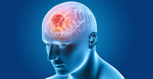
Fig.1. Understanding Brain Tumours Available at: https://www.yashodahospitals.com/blog/brain-tumours symptoms-causes-treatment/
1.3 MRI Images Exam Analysis
Definition of MRI
Magnetic Resonance Imaging (MRI) is a non-invasive imaging technology that produces 3D detailed anatomical images. It is used for diagnosis, disease detection and treatment monitoring.
Accordingly, to Peter Lam from Medical News Today, an MRI scanner contains two powerful magnets, which are the most important parts of the equipment.
The scientific part behind is how it works, being more specific, it works by a radiofrequency current that is pulsed through the patient and the protons are stimulated, and when the radiofrequency is turned off, the MRI sensors are able to detect the energy released on the protons that realign with the magnetic field.
The process is the patient is placed inside a long magnet and remains during the imaging processing in order to obtain an MRI image.
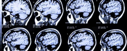
Fig.2. MRI Image for the Brain, Available at: https://www.myvmc.com/investigations/3d-magnetic-resonance imaging-3d-mri/
Use Cases
The MRI can be used for:
-Anomalies of the brain
-Tumor in general and other anomalies in different parts of the body
-Breast Cancer
-Certain types of heart problems
-Suspected uterine anomalies
-Diseases of the liver and other abdominal organs.
There are special types of MRI such as:
1.Magnetic Resonance Angiography (MRA) and Magnetic Resonance Venography (MRV) – useful to help the surgeon plan an operation.
2.Magnetic Resonance Spectroscopy (MRS) – it measures biochemical changes in the area of the brain.
3.Magnetic Resonance Perfusion – it is used after the treatment to determine if an area that still looks abnormal is remaining the tumour or not.
4.Functional MRI (fMRI) – it is used to determine which part of the brain to avoid when planning surgery or radiation therapy.
1.4 Convolutional Neural Networks
Convolutional Neural Networks (CNN) is a deep learning algorithm that takes an input and learns its various aspects and objects of the image and after its training is capable to differentiate one from the other according to the purpose. The most common use cases are in computer vision for classification, object detection and segmentation of images datasets.
CNN can have tens or hundreds of layers that can learn to detect different features, like other neural networks, composed of input layers, hidden layers and output layers. The most common layers are
1.Convolution – the input images pass through a set of convolutional filters.
2.Rectified Linear Unit (ReLu) – it is an activation function where only the activated features are carried into the next layer.
3.Pooling – Perform non-linear downsampling, reducing the parameters that the network has to learn.
Convolution Operation
It is an operation of two functions of real valued arguments.it leverages three important ideas that can improve a machine learning system which is sparse interactions, parameter sharing and equivariant representation, in other words, it provides a means for working with inputs of variable sizes.
Pooling Operation
A typical CNN consists of three stages, the first the layer performs several convolutions in parallel to produce a set of linear activations. Second, each linear activation runs through a non-linear activation function, third, a pooling function is used to modify the output of the layer further.
In other words, pooling supports to make the representation invariant to small translations of the input. It replaces the output of the net at a certain location with a summary statistic of nearby outputs.
Pooling it is very handy in some situations as image classifications for example but can be not the best solution for some architecture types such as autoencoders and Boltzmann Machines.
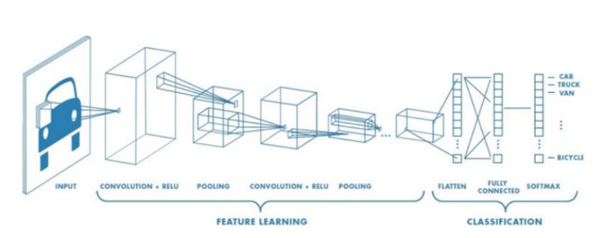
Fig.3. Traditional CNN Architecture, Available at https://medium.com/@hannahfarrugia/convolutional-neural networks-cnn-and-use-cases-in-health-b3b0fd75bcca
There are many architectures of CNN available that can be performed in many cases, the most knowns are
1.LeNet
2.AlexNet
3.VGGNet
4.GoogLenet
5.ResNet
Successful CNN applications
CNN usually are applied in computer vision and image recognition tasks such as: -OCR and image recognition
-Social Media face recognition
-Image Analysis in Medicine
-Objects Detection in self-driving cars
Face Detection – it is used to detect faces in image, it can detect features such as eyes, nose, mouth with great accuracy.
Face Emotion Recognition – it can classify facial expressions such as anger, sadness, or happiness.
Object Detection – It is used to localize and identify objects within images, also can create different views of those objects such as for use in drones and autonomous vehicles.
Autonomous Cars – It enables vehicles to detect obstacles or interpret street signs.
Cancer Detection – It can detect cancer in medical images such as mammograms and CT scans.
X-Ray Image Analysis – It can identify tumours or other abnormalities in X-Ray images and determine which area of an X-Ray image contains a tumour or other abnormalities such as fractures bones for example.
3D Medical Image Segmentation – It can segment medical imaging scans, such as MRI Images.
Biometric Authentication – It can be used for biometric authentication of user identity by associating certain physical characteristics with the person’s face.
Other tasks, it can be used into different segments that can benefit from CNN development, and it can be applied to different problems. This list is just an illustration of successful cases but is not the limit of it.
1.5 CNN Segmentation
CNN Segmentation divides a visual input into segments, which are made of sets of one or more pixels. Image segmentation sorts pixels into larger components and eliminates the need to consider pixels as a unit, the process of image segmentation starts with the definition of small regions on an that should not be divided, this region is called seeds and the position of it defines the tiles.
The architecture for segmentation utilizes the encoder and decoder technique model, where the encoder is used to encode the representation to be sent through the network and the decoder to decode the representation back.
Images Segmentations can be divided into:
1.Semantic Segmentation – classifies the image like small groups of pixels that are likely to belong to the same object, in other words, it means all pixels correspond to a class given to the same pixel value.
2.Instance Segmentation – each instance of an object is identified separately. Each object in the image is identified differently. The pixels correspond to each instance or object of the class by giving unique values; these values can range from 0 to N, where N refers to the total numbers of objects in the image.
By analyzing the two techniques, semantic segmentation can be applied when not necessarily multi-classification tasks or a very meticulous segmentation, while instance segmentation can be very handy to classify multiple objects or different localizations, and for a 3D Image Analysis, specially for a brain segmentation where accuracy is highly important is the indicated technique approach.
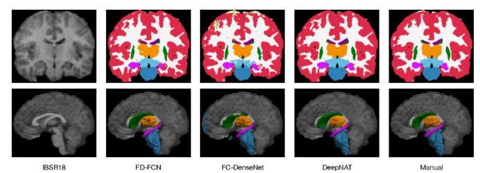
Fig.4. Instance Segmentation in MRI Brain Images, Available at: https://www.semanticscholar.org/paper/FD FCN%3A-3D-Fully-Dense-and-Fully-Convolutional-for-Yang Zhang/e07914b3103a0c49fafe2d6bf52f1435d8c2c67b
1.6 Fully Convolutional Network (FCN)
While a typical CNN is not fully convolutional, a FCN (Fully Convolutional Network) is a neural network that only performs convolution, subsampling or up sampling operation. FCN is a CNN without a fully connected layer.
Other characteristic of FCN is that does not contain “dense” layers as in traditional CNN, but instead contains 1×1 convolutions that perform the task of fully connected layers, which it means, there are fewer parameters, as a result the networks are faster to train, and a handle a wide range of image sizes since all connections are local.
Unpooling (Network Upsampling) -While pooling converts a patch of values to a single value, unpooling does the opposite, by converting a single into a patch of values
Transposed Convolution – It is used to upsample the reduced resolution feature back to its resolution, a set of strides and padding values is learned to obtain the final output from the lower resolutions.
Skip Connections – It is applied in the Upsampling stage from the earlier layers to provide enough information to later layers to generate accurate segmentation boundaries.
Example of FCN
U-Net and its variations is an example of a convolution network, that is used for semantic segmentation.
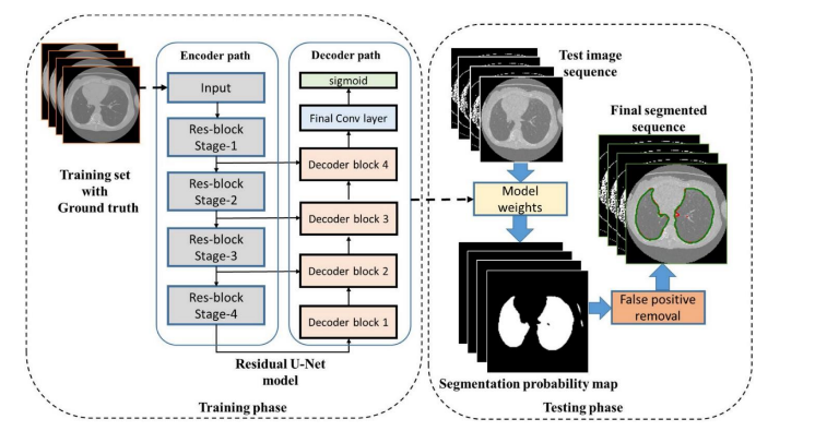
Fig.5. Proposed Residual U-Net for lung CT segmentation, Available at : https://medium.com/codex/architectures for-medical-image-segmentation-part-3-residual-unet-ac5a4ca4212d
1.7 U Net Model for 3D Image Analysis
U-Net Architecture
U-Net Architecture was specially designed for Biomedical Image Segmentation in 2015 by Olof Ronnebeger.Today it is applied into other problems that require semantic segmentation tasks. It is a fully convolutional neural network that can learn from a few training examples.
It has a U-shape encoder-decoder architecture, with four encoder and decoder blocks connected. Some researchers have tried some adjustments in this architecture, one new utilization was adding dropout together with the ReLu activation function, this modification helps the network learn from different representations and avoids overfitting.
Another modification made in the architecture was the addition of a batch normalization layer between the convolution layer and the ReLu, with the objective to make the network more stable during the training.
Encoder Network
The encoder network behaves as a feature extractor and learns the abstract representation of the input image through a sequence of the encoder blocks. Each encoder block has two 3×3 convolutions, with each convolution followed by an activation function, usually it is applied to ReLu.
The output of ReLu behaves as skip connection for the corresponding decoder blocker, then , it follows a 2×2 max-pooling , to reduce the feature maps to half, by utilizing the spatial dimensions. This technique decreases the number of trainable parameters and reduces the computational cost.
Bridge
Connecting the encoder and decoder network, it has 3×3 convolutions followed by a ReLu activation function, with the objective to complete the flow of information.
Decoder Network
The state-of-the-art happens here, where the decoder network takes the abstract representation and generates a semantic segmentation. The decoder initializes with a 2×2 transpose convolution, then concatenate with the corresponding skip connection feature map from the encoder block, to finalize, it is used two 3×3 convolution, with each convolution followed by an activation, usually used ReLu here too.
As output, it uses 1×1 convolution with sigmoid activation function, where it will give the segmentation representing the classification.
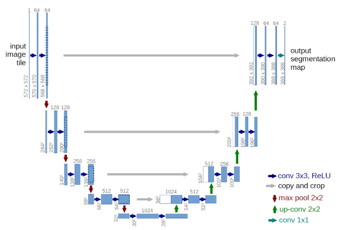
Fig.6. U-Net Architecture. Each blue box corresponds to a multi-channel feature map, the number of channels can be visualized on the top of the box, while the white boxes represent copied feature maps.
Available at: https://lmb.informatik.uni-freiburg.de/people/ronneber/u-net/
Attention U-Net Architecture
This architecture can be applied in natural language processing and natural image analysis, but it is being used for medical image segmentation as well, due to automatically learning on target structures and variation of the shapes and sizes.
The Attention context was introduced in “Need to pay attention” by Jetley et al. , where it trains an end-to-end attention module.
Attention Gates
To improve segmentation performance, the proposal by Khened et al. and Roth et al. was to integrate attention gates on the top of the U-Net Architecture, without need to train additional models.
As a result, the attention gate improved the model sensitivity and accuracy without using computation overhead.
This technique is applied before the concatenation operation to merge only relevant activation, allowing model parameters in prior layers to be updated based on spatial regions that are relevant to a given task.
Grid-based gating
It is used to improve the attention mechanism; when implemented, the gating signal is not a single global vector for all image pixels, but a grid signal conditioned to image spatial information.
When this method is applied, it allows attention coefficients to be more specific to local regions, the results is a better performance compared to gating based on a global feature vector.
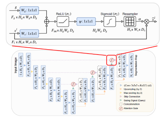
Fig.7. Attention U-Net Architecture. Available at: https://sh-tsang.medium.com/review-attention-u-net-learning where-to-look-for-the-pancreas-biomedical-image-segmentation-e5f4699daf9f
Residual U-Net Architecture
The residual U-Net was created for image segmentation cases in recent years, with the objective to introduce the shortcut connection, to solve the problem of degradation. The main reason for that was because very deep networks were not capable of handling the problem of degradation.
Deep Residual U-Nets is a great architecture for complex image analysis tasks, being successfully used in applications such as breast cancer, prostate cancer, brain tissue quantification, brain structure mapping, etc.
This technique improves the flow of information in the network, by reformulating the layers as learning residual functions to the layer inputs. This approach solves the degradation problem in a deep network.
It contains a set of residual blocks, each of which consists of stacked layers such as batch normalization, ReLu activation and weight layer. Shortcut connection means skips one or more layers in the network.
When a residual unit is built, then the next step is to build a very deep convolutional encoder decoder by stacking residual units.
Four stages are used in the encoder and decoder part and each stage uses residual blocks. The stage is considered a unit where stage 1 has 3 units, stage 2 and 3 have 4 and 6 units respectively and stage 4 has 3 units.
Encoder Part
The architecture has a total of 50 convolutional layers in the encoder part, the convolution operations are performed in each block.
The input image is resized to 128×128, followed by a batch normalization, then is carried with filter side 3×3.
Decoder Part
Consists of Up Sampling layer, concatenation layer followed by stack convolution, batch normalization and ReLu activation. Lastly, a 1×1 convolutional layer followed by a sigmoid activation function. This part is used to generate the probability score at the output of the model.
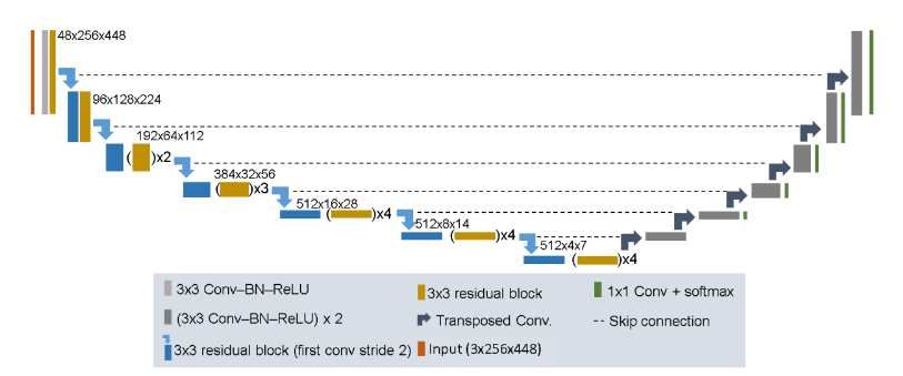
Fig.8. Residual U-Net Architecture. Available at: https://www.arxiv-vanity.com/papers/2004.12668/
2. Description of the technique/procedure analyzed
2.1 Experiments
A GPU is interesting to have to perform the task, due to the high complexity of the model and size of the dataset.
GPU performs faster calculations due to its parallel architecture, while CPU takes far longer time to deliver the results of the same training.
Keras/Tensorflow was selected for the experiment since it is faster to learn and popular for commercial environments and producing solutions. Anyway, it is interesting to experiment with other frameworks such as Pytorch, which is known between academics and for research environments, it has a higher learning curve than other competitors.
Those are not the only frameworks available on the market, it has other options but the most acceptable and utilized by the community are the ones mentioned.
For code execution, anaconda is selected using jupyter notebook, the libraries imported are numpy, pandas, tensorflow, keras, scipy, scikit-learn and installed properly.
The process for the implementation is:
1.Import the libraries that are going to be used in the task.
2.Dataset downloaded, divided, and organized into 2 sets, training and test set respectively
3.Each specific Architecture separately into different cell (U-Net, Attention U-Net and Residual U-Net individually with its own variation) , only parameter has kept the same is Optimizer = Adam and learning rate = 0.001
4.After the dataset is prepared, the next step is the model implementation receiving the following hyperparameters.
Batch Size = 64, Epochs = 5, Validation Steps = 200//, Steps per Epoch = 800//batch 5.Evaluation methods, which is the same for each architecture and classified into: Loss Function = binary_crossentropy , metrics = accuracy and dice coefficient
The evaluation metrics will bring the necessary information after the training for each architecture and then it is possible to analyze it on a table sheet and do the comparison between the results.
2.2 Dataset
The BraTz 2021 dataset contains MRI scans of glioma, pathologically confirmed diagnosis and available open source for training, validation, testing with different models
All the datasets have been annotated by specialists, and by one of the four rates, classified as:
➔ GD Enhancing Tumor (ET Label 4)
➔ Peritumoral edematous/invaded tissue (ED Label 2)
➔ Necrotic tumor core (NCR Label 1)
The format files are NIfTI files (.nii.gz) ,with the collaboration of many institutions, that provided various scanners and different clinical protocols to enrich the quality of the dataset. The division of the files are native (T1), post-contrast T1 – weighted (T1GD), T2-Weighted (T2) and T2 fluid attenuated inversion recovery.
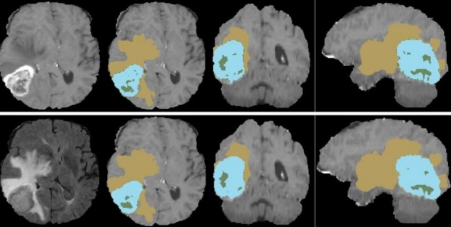
Fig.9. Sample of the dataset. Available at: https://www.kaggle.com/datasets/dschettler8845/brats-2021- task1
2.3 Training
As a training, after the libraries are imported, the next is to download and extract the images into a new file. A function called Data_Preprocessing it utilizes numpy to divide the datasets in Flair,T1,T1ce,T2 and GT , which is a classification of the images accordingly to its particular condition and already defined by the dataset which was classified by specialists, so in this steps the objective is just to separate the images by its divisions.
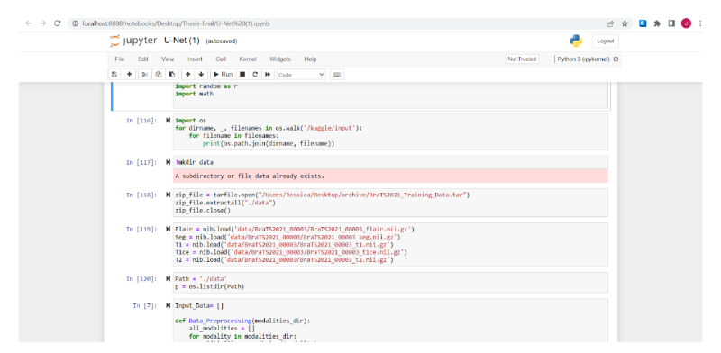
Fig.10. Dataset downloading and preparation of the data, printed by the author
Next function is Data_Concatenate where it receives the parameter called input_data , the objective here is to concatenate the data, then is converted into float type and receives the division as the training set and testing set.
As the traditional way is divided into X_train, X_test, Y_train , Y_test = train_test_split (TR,TRL ## Here are numpy arrays commonly ## ,test_size , random_state).
It receives the slices by utilizing tensorflow framework and it is checked to assure if all the data is in the same format for the training.
Data augmentation is performed by changing the brightness, Gama, crop and rotation, with the intention to produce a better data quality and resolution in the moment of the training.
1. U-Net Model
The step for data preparation is completed, then can start with the architecture U-Net Model ##At this part it will receive the updates for the next training with the other U-Net variants ##
The U-Net model first receives a convolution function defining the kernel size, padding, strides, batch normalization and ReLu activation function.
Next is the Model function, the first convolution receives the input and the maxpooling, the second till fourth convolution increase values and receives maxpooling again, from the fifth till eighth convolution it adds the upsampling method, the ninth convolution is the output, and it has sigmoid activation function to produce the final outcome.
2. Attention U-Net Model
It starts with a function gating_signal (for the attention unit), where it defines the batch normalization and ReLu activation function as parameters.
Next is the function called attention_block, that is based on soft attention, where it will receive the kernel size, strides, passing and upsampling.
#Downsampling
Here it comes the bigger structure of the model architecture, where a function called Attention_UNet receives a dropout = 0.2 (this was mentioned before that it can be utilized to increase the performance of the model) , downsampling layers divided into four steps receiving convolutional parameters and maxpooling, the fifth variable it ends by receiving only convolutional parameters.
#Upsampling
Here starts the state-of-the-art, it is divided into four gates, where it will receive the gating_signal and attention_block that was defined as functions before.As completion of the variable it receives the sigmoid activation function as final outcome for the model.
3. Residual U-Net Model
This architecture starts by defining its filters, kernel size, upsample size, batch normalization and dropout=0.2
#Downsampling
Starts with four stages receiving the parameters defined above and one layer of maxpooling in each stage.The fifth state and last does not receive maxpooling as the difference of the model shape.
#Upsampling
It has four stages as well, upsample size, layers concatenation, kernel size , batch normalization , filters and dropout.
As the fifth stage receives the final convolutional, together with a sigmoid activation function
Post- Model Architecture
With the model created then can check the summary for the model, the results for the U-Net is the same by having a total parameters: 3.297.792 , Trainable parameters: 3.294.849 , Non Trainable parameters: 2,944
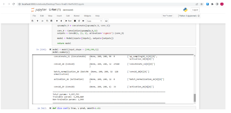
Fig.11. Model Summarization for Illustration, printed by the author
For the compilation for the model the optimizer selected is Adam at learning rate = 0.001 , binary cross-entropy as loss function , metrics for evaluation = accuracy and dice coefficient.
The model training is at this stage, when it applied the model.fit to receive data training, steps per epoch, validation steps and number of the epochs.
After training the model, the output is ready to be visualized as quantitative and plotted by graphic methods.
3.Extensions (improvements and future of lines of research)
3.1 Results
First result that got attention was the data visualization before and after the data augmentation for the images, it is very clear that the image after this treatment, got a better resolution and brightness, this can be very handy to support the algorithm to improve its accuracy.
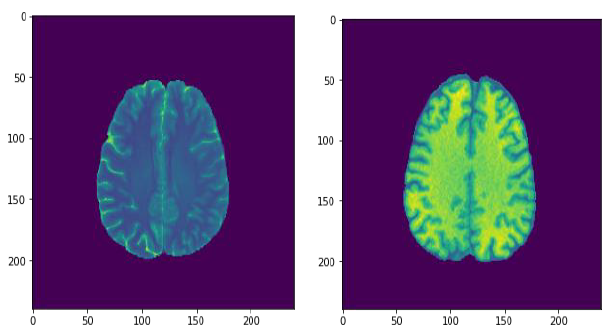
Fig.12. Comparison of the image resolution before and after data augmentation, printed by the author
Other observation made, is that some tasks require a bigger number of epochs to reach a good performance, the understanding here is not only the quality and size of dataset makes the difference, but also the architecture model that is going to be utilized.
U-Net models and its variants performs and fit into the task very well , and the difference as performance regarding the speed , the traditional U-Net is faster than the others, but when it comes as final output of performance in terms of accuracy and dice coefficient there are very small difference, but for a brain segmentation case, it is critical and required to reach the highest accuracy possible in the training.
The image below clearly shows a good resolution, segmentation and has only received 5 number of epochs during the training, which demonstrates a sign that U-Net and variants are interesting models to be applied in the Medical Image Analysis Segment.
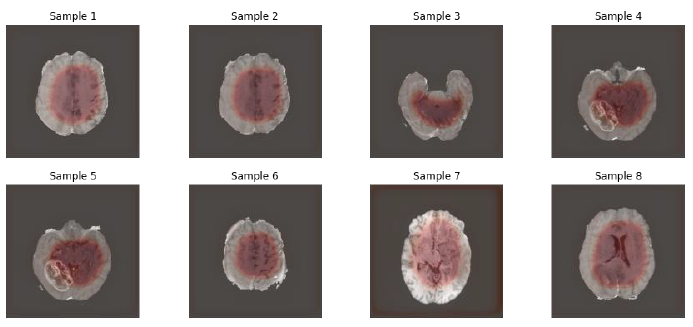
Fig.13. Outputs after training completed, printed by the author
3.2 Performance of the models
This stage is to compare the performance for U-Net, Attention U-Net and Residual U-Net individually after the training and compare the results, with the objective to evaluate the performance, which is the final objective of the proposal.
As the accuracy happens during the training of each epoch , it improves over the time and with more training of the model , all the variants reach a good performance and the differentiation as accuracy metric is very small as it shows in the sheet table , as the Attention U-Net receives the best performance overall , but the Residual U-Net it is very close to achieve the same results, while the U-Net performed well but it is a bit way from the other two variants, but still the number differentiation is minimum as well.
| Models | Accuracy | Median Overall |
| U-Net | 0.965 ; 0.9 ; 0.882 | 0,9156 |
| Att-U-Net | 0.966 ; 0.905 ; 0.893 | 0,9213 |
| Res-U-Net | 0.964 ; 0.903; 0.893 | 0,92 |
The second metric to evaluate the performance is the dice coefficient, it is performed during the training while the number of epochs is running, and it works in the same way it improves over time and by training the model, this table sheet demonstrates mean dice coefficient over all the model’s architectures and again it shows a similar result as the accuracy. All the U-Net variants perform very well, but the best overall is the Attention U-Net followed closely by Residual U-Net and lastly U-Net, but with no underestimation at all.
| Models | Mean Dice Coef |
| U-Net | 0.9100 |
| Att-U-Net | 0.9110 |
| Res-U_Net | 0.9103 |
3.3 Discussion
It was observed that it has increased the research of Artificial Intelligence in the Medical Analysis Images, not only for MRI exams, but also X-Ray and CT and applied into different cases mostly for automation of diagnosis.
The algorithms are learning from the patterns how to identify based on the training, if a person has determined disease or not, there are papers available not only for brain segmentation, but for other types of cancers located in the prostate, pancreas and other organs.
Besides that, even with the advance of AI still it has limitations, being applied to only a specific problem, in other words, it creates a specialist system, but not a general system that is capable of identifying all diagnoses in multiple regions at once.
The fully convolutional networks and segmentation techniques are very handy to perform this task because a precision is required in the localization of these tumors. Perhaps, the U-Net and its variants are the most used in the medical field for segmentation but are not the only ones available for training a model, but naturally the model will need to follow some principals as the image segmentation for example.
The interesting part to use the U-Net is because is encoder-decoder type , and usually deal very well with a large dataset that is enough to train a model and the type of formats and size this files usually have, a traditional CNN may not be enough to handle it with a good accuracy , adding also how this architectures treats a image for learning during the process is very meticulous and exactly what is necessary for this kind of task where every single details should not be lost during the analysis.
The brain segmentation is a challenging task, because of the necessity of the precision on the evaluations, and where error can be critical as it is dealing with humans’ life.
Although these models are explainable and work in a very objective way, there is still the idea to be a black box, still there is the necessity to somehow understand completely how these algorithms really learn and assure that it will work with efficiency at all the time.
The advance of science on AI has increased exponentially, but still there are many mechanisms that need and might be improved in the future, regarding hardware’s, new model’s architectures, new mathematical equations, new discoveries in the neuroscience that can help these intelligent systems improve its methods and reach to a new stage inside the Artificial Intelligence Field.
The integration of AI in medicine is not closed only to image segmentations, and there are new technologies emerging in the segment such as Da Vinci robot that supports the doctors on the surgery, machine learning algorithms that can identify some diagnosis, treatments and preventions, Robot assistants and even Internet of things in the healthcare.
It is just the beginning of the context, and the objective was not to close the subject, instead open the door for new forms to create new modes with different approaches.
3.4 Conclusion and future of the work
As a conclusion, the experiment was performed using U-Net, Attention U-Net and Residual U-Net for the brain tumor segmentation case utilizing the BraTz 2021 dataset, which is open source and available on Kaggle for training models and incentives the research on the segment.
It started by defining how the brain tumors can start, classifications, diagnosis and treatment, then as part of diagnosis is the MRI (Magnetic Resonance Image), which provides high resolution images, to support the specialists to identify with precision where the tumors is located.
As the problem is defined, the next approach is to introduce the part of Artificial Intelligence can support in this case, which a CNN (Convolutional Neural Network) is detailed and followed by instance segmentation and FCN (Fully convolutional Networks), which is the theory that comes the U-Net and its variants and it is generally used for medical analysis segmentation.
It reaches the core by detailing and explaining how this encoder-decoder model works individually, as each U-Net variant is very similar, but it has some modifications in its architecture.
By carrying out this information, it is ready to do the experiment and evaluate the performance for each model. The entire implementation received the same dataset and hyperparameters such as number of epochs, batch size, batch normalization, optimizer, learning rate and final metrics.
Based on the experiment, the U-Net presents a great performance even with small number of epochs, which demonstrates it is a very good model architecture, but as final performance in terms of accuracy and dice coefficient Attention U-Net takes the advantage over the other variants, but with a very small difference in accuracy as it shows in a table sheet in the final performance stage.
The future of work for Artificial Intelligence is promising in the Medical Analysis Image as the U-Net and its variants, but it is not the final results, performance or architecture.
It is interesting to try new learning rates, number of epochs, differentiate the datasets, different metrics for evaluations, including adding other types of U-Nets or other model architecture, in other words, try to solve the same problem in different ways to understand the results from different perspectives and what it changes during the way.
Lastly, it is highly encourage and worth the attention for research and development in the brain segmentation case , as in other types of cancer images and diagnosis, as the U-Nets can be utilized for other tasks as well , and the incentive to improve and create new architecture models, GPU and frameworks that can make the AI one day support the doctors in faster diagnosis and treatments, and as result a better efficiency in the medicine sector.
3.5 References
[1] American Association of Neurological Surgeons, available at: aans.org , (accessed:01 august 2022).
[2] Data Science Academy,(2016) “Deep Learning Book” , available at: www.datascienceacademy/book , (accessed: 16 July 2022).
[3] Ekman K.,(2022) “Learning Deep Learning”, Edition 1 , Deep Learning Institute , Pearson.
[4] Feifan W. , Jiang R.,Zheng L.,Meng C. , Biswal B. ,(2020) “3D U-Net Based Brain Tumor Segmentation and Survival Days “ , available at: arxiv.org/abs/1909.12901 , (accessed:10 july 2022).
[5] Futrega M. , Milesi A, Ribalta P, (2021) ”Optmized U-Net for Brain Tumor Segmentation “,available at:arxiv.org/abs/2110.03352,(accessed:16 july 2022).
[6] Goodfellow I. , Bengio Y. , Courville , (2016) “Deep Learning” , Massachusetts Institute of Technology
[7] Mohammed H, Davy A. , Farly D, Biad A, Courville A. , Bengio Y. , Pal C. , Jadoin P. , Larochele H. ,(2016) “Brain Tumor Segmentation with Deep Neural Networks” , available at:arxiv.org/abs/1505.03540, (accessed:10 july 2022)
[8] Siddique N, (2020) “U-Net and its variants for medical image segmentation: theory and applications” , available at: arxiv.2011.01118, (accessed:18 august 2022).
[9] Simon H. , (2008) , “Redes Neurais – Principios e praticas” , Edition 1 , Bookman
[10] Stuart J. , Norvig P. , (2010) , “Artificial Intelligence – A modern Approach”,Edition 2 , Pearson.
[11] Witchayakan W, (2021) “U-Net with Pytorch”, available at: kaggle.com/code/witwitchayakarn/u-net-with-pytorch ,(accessed: 19 august 2022)
1Master in Artificial Intelligence and Deep Learning