REGISTRO DOI: 10.5281/zenodo.10495482
Ronaldo Nakamoto1, *;
Pedro Estigarribia Pompílio1, †;
Claudio Bastos Silva1, †;
Bruno Pohlot Ricobom1, †;
Horacio Tertuliano Filho1, †
Abstract
Transmitter and receiver antennas play a pivotal role in wireless systems, exerting a significant influence on overall receiver sensitivity and link performance. They represent integral and autonomous elements within any wireless communication system. With the growing demand for connectivity in wireless networks, the proliferation of the Internet of Things (IoT) concept, and the wide array of applications, such as radiofrequency identification, antennas have found versatile applications. Antennas have become essential allies in the pursuit of enhanced connectivity, whether for data exchange or the transmission of electromagnetic signals. The dimensions of antennas can pose challenges, especially as equipment continues to shrink in size, with antenna dimensions directly impacting device proportions. Printed antennas hold significant value in scenarios where minimizing component size is imperative without compromising performance. This research aims to design and simulate antennas, aiming to assess their advantages and disadvantages compared to conventional antenna models used in UHF band wireless systems. Index Terms—Antenna radiation patterns, antenna measurement, fractal antennas, simulation.
I. INTRODUCTION
The pursuit of maximum efficiency in printed antennas entails a thorough analytical study to accurately determine the factors that influence resonance and radiation capability across various operating frequencies. This extends to comparisons with physically modified antennas, achieved through techniques like recursion or the introduction of fractal patterns[1].
The present research endeavors to design a patch antenna with fractal geometry, specifically the Sierpinski Carpet, across orders zero, one, two, and three. These antennas will be fabricated on a double-sided printed circuit board for operation within the 915 MHz range.
Furthermore, the research delves into the electromagnetic behavior of the antenna, covering aspects like radiation, and reflection patterns, gain, as well as its advantages and functionalities compared to other commonly used printed antennas, such as those with rectangular and circular geometries printed on circuits.
II. THE PATCH ANTENNAS
Patch antennas fall under the category of aperture antennas, where the radiation source is confined to a defined surface within a medium, which, in this case, is the copper area that constitutes the antenna.
These antennas are typically constructed using printed circuit boards, consisting of a conductive metal layer sandwiched between dielectric material on a ground plane. The shape of patch antennas can vary depending on their intended application, and each geometry will inherently affect the antenna’s behavior. The radiation mechanism in microstrip antennas is closely tied to a phenomenon known as edge fields. This electromagnetic effect leads to a shift in the resonance point, effectively simulating an antenna with a greater length than its physical dimensions. When observing a square patch microstrip antenna from the side, the ends of the patch create discontinuities in the conductor, akin to open-circuit points. At these points, the impedance at the edges of the patch tends toward infinity (in practical terms, they reach values on the order of 300 Ohms), and the current is nearly zero. This unique behavior leads to the generation of electric fields with edge effects. The fields near the surface of the patch are all oriented in the same direction, combining in phase adding up coherently and contributing to antenna radiation. A similar effect occurs with the current, but an equal current flows in the opposite direction through the ground plane, which cancels out the radiation [2].
A. Fractal Geometry
The term ‘fractal’ denotes a creation or form that exhibits fragmentation, irregularity, and a lack of strict adherence to conventional rules. It is employed to characterize intricate shapes that share similarities with their own geometric structure. Additionally, it can be defined as a collection of forms that comprise a recursive cascade.
Rooted in the concept of infinity, fractals expand the boundaries of classical geometry, which traditionally revolves around points, lines, and circles, into the realm of irregularity, fragmentation, singularity, and uniqueness. This broader perspective allows for the description of a wide range of patterns, geometric shapes, and other elements found in nature. For a geometric shape to be classified as fractal, it must possess specific attributes, including self-similarity, infinite complexity, intricate fine structure and simplicity in its formation rules [3].
1) Self-Similarity and Infinite Complexity:
To characterize a fractal, it’s crucial that a part of the figure resembles a larger portion of the whole figure, a concept known as self-similarity. This self-resemblance occurs through a process of recursion within the patterns. Self-similarity can manifest in two distinct forms: exact and approximate, or statistical. Exact self-similarity is a characteristic property found primarily in mathematically generated fractals, where the entire set is crafted through iterative processes, resulting in the formation of tiny, perfect replicas of themselves, as exemplified by instances like the Sierpinski Carpet and the Koch curve [4].
2) Intricate Fine Structure:
This characteristic ensures that the level of detail remains consistent even when examining a minute portion of the geometric shape. It enables one to discover the same richness of details within a part of the figure as we would find in the whole. As an illustration, let’s consider the Sierpinski Carpet of order 3, Fig.1 (Fractal Order Three) [5].
3) Simplicity in its Rules of Formation:
The creation of a fractal figure can be achieved through iterative, recursive, or stochastic methods. Despite the richness of detail and the complexity of their structures, these figures can be generated using relatively straightforward techniques. However, unlike classical geometric figures that can be precisely described through equations, such as those in Euclidean geometry that are directly associated with concepts like height, width, and length, fractal shapes often defy such simple mathematical representation. Instead,
they exhibit irregular shapes and fractional dimensions [6].
B. Sierpinski Carpet
The rectangular Sierpinski Carpet (third order) is a flat shape created through an iterative process of dividing a rectangle into nine identical rectangles and then removing the central one, leaving only eight rectangles as shown in Fig. 1 (Fractal Order Three) [7]-[8].
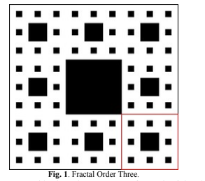
The same procedure is repeated in the subsequent step for each of the eight new rectangles and so forth. This fractal is categorized as a geometric one, as it possesses all the defining characteristics. When observing the highlighted section, a level of detail similar to that of the entire figure is achieved.
C. Fractals in Telecommunications
Fractal geometries are defined through experimental parameters, and their level of complexity often defies precise mathematical description. Understanding them involves practical studies and mathematical deductions, particularly regarding their recursive nature. Experimental studies guide the parameters in fractal design, leading to desired outcomes.
A key attribute of fractals is their fractional dimension, which measures how efficiently the object occupies space. Fractal curves are mathematically capable of more efficient space coverage than standard Euclidean surfaces, a critical aspect in antenna miniaturization.
Fractal antennas offer a range of advantages, such as multi-band performance at non-harmonic frequencies and input impedance matching, simplifying circuit design. Additionally, their far-field radiation patterns tend to align with the operating frequency.
The complexity of fractal antennas derives from the intricate geometries rooted in basic shapes, with complexity increasing as the number of fractal iterations rises.
Leveraging recursion and the potential for size reduction, significant efforts have been devoted to implementing multi-band antennas for cellular telephony [9]-[10].
III. BASIS OF ANTENNA GEOMETRY
A. Rectangular and Zero Order Fractal
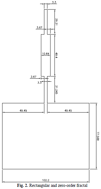
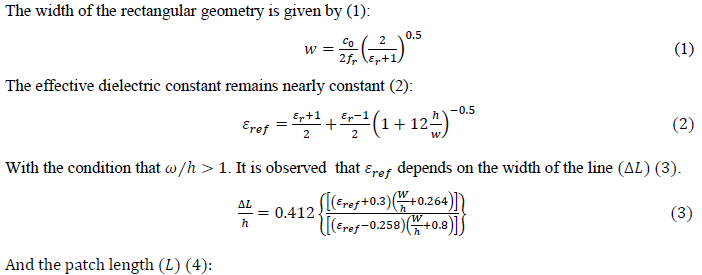
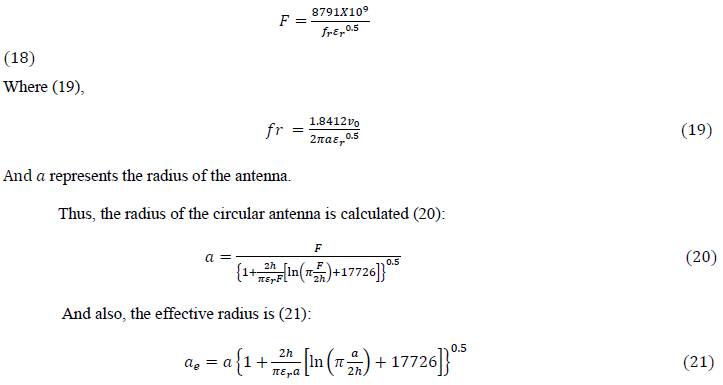
For the rectangular patch illustrated in Fig. 2 (Rectangular and zero-order Fractal), equivalent to the zero-order fractal [11]-[12], the width of the rectangular geometry is determined by the electromagnetic wave velocity in a vacuum (c0), the substrate’s dielectric constant (εr), and the resonance frequency (fr), which, in this case, is set at 915 MHz.
D. Fractal Geometry
The Sierpinski carpet begins with the initial rectangular shape, and its subsequent dimensions are proportional to the largest rectangle ́s limits. During each iteration, the measurements and positions of the elements to be removed from the metallic substrate are calculated. L represents the size of the main square, and W represents the size of the other squares. L represents the side length of the squares in the nth iteration, where ” n ” is the iteration number. The W proportion is determined using the formula Ln = n⁄3, which means that, in each subsequent iteration, the size of the squares is reduced to one-third of the size of the
previous iteration. This helps define the specific dimensions of the elements at each stage of the Sierpinski carpet fractal generation process. Following this criterion, there is a sequential reduction in the dimensions of the elements with each iteration and an increase in the quantity Nn of these modified elements [2]-[14].
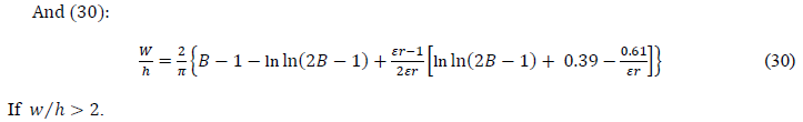
Let r represent the number of divisions of L, M be the proportionality factor for each side of the squares (31), and Q be the proportionality factor for the non-removable elements at each iteration (32) and (33). These values are:
For constructing a Sierpinski carpet with r = 3, the approximate Hausdorff dimension is 1.8928,
and the available area for the next iterations is determined by (34):
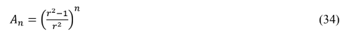
In the construction, Fractal Geometries had their dimensional adjustments following the theoretical methodology for the rectangular geometry, which is equivalent to the Zero Order.
A portion of the substrate referred to as M2 is removed from each new subset of elements obtained in successive iterations for this construction. As the number of iterations increases, it leads to a reduction in the available area of the main conductor and an increase in power loss due to the Joule effect. This presents one of the limiting factors on the number of possible iterations. Another limitation relates to the impact of iterations on operating frequencies. With higher iteration orders, the dimensions of the removed portions decrease and start to affect progressively smaller wavelengths. Beyond a certain order, the effects of fractals on the antenna’s performance become noticeable at higher frequencies [15]. This makes it
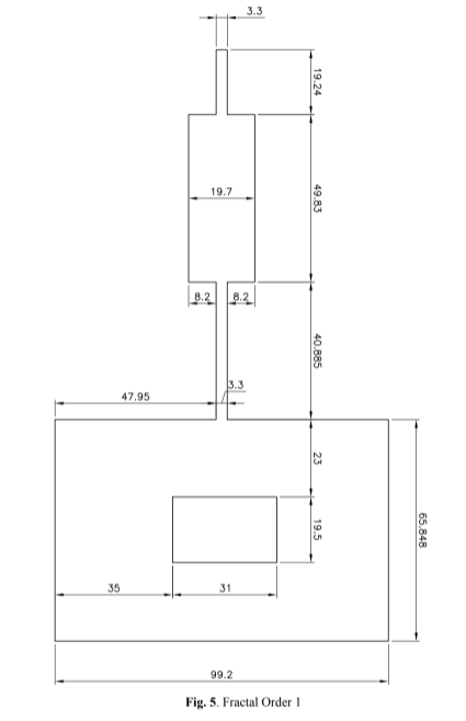
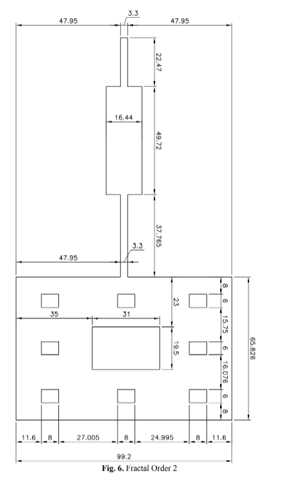
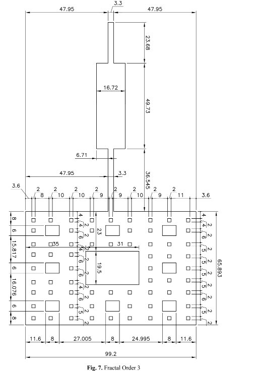
challenging to reproduce the required dimension accuracy. In the construction of Fractal Geometries, their dimensional adjustments followed the theoretical methodology for rectangular geometry, which is equivalent to the Zero Order. Fig. 5 (Fractal Order 1), Fig. 6 (Fractal Order 2) and Fig. 7 (Fractal Order 3) display the fractal antennas with orders one, two, and three, respectively.
IV. SIMULATIONS
For enhanced accuracy in the antenna development process, from mathematical formulation to real device assembly, it is advisable to simulate the antennas to obtain data and model the patch dimensions.
Ansys HFSS, a software designed for high-frequency simulations, including antennas and microwave components like connectors, filters, and high-speed interconnectors, was used. This software finds applications in the development of radar systems, satellites, and IoT devices.
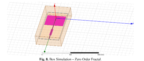
A. Rectangular geometry In this simulation, the dimensions of the Patch antenna can be defined within software simulation parameters, considering the present radiations. The relevant parameters are input into the software based on the project conditions like displayed in Fig. 8 (Box Simulation – Zero Order Fractal). Fig. 8. Box Simulation – Zero Order Fractal.
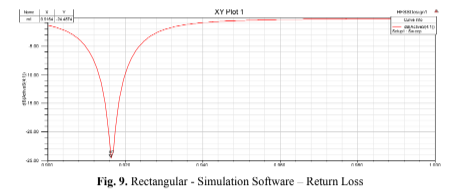
The Fig. 9 (Rectangular – Simulation Software – Return Loss) displays the plotted return loss at
different frequencies for the analyzed antenna. When this loss reaches a minimum value, there is no reflection in the Microstrip Line, enabling the transmission of current and voltage almost in its entirety. This also indicates impedance matching, allowing for practically complete radiation and optimized performance. In this case, impedance matching is observed at a frequency of 913.2894 MHz, as the return loss was minimal. At this frequency, the input impedance is very close to 50 Ohms.
In Fig. 10 (Rectangular Geometry – Smith Chart), using the Smith Chart, it is possible to associate the reflection coefficients with the resonant frequency. In the center of the circle, the coefficient is null and increases with distance [16].
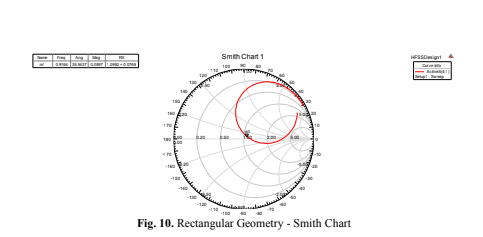
At the frequency of 0.9133 GHz, it is almost centered, indicating near-zero reflection coefficient
and impedance matching.
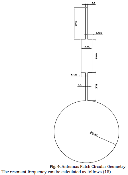
B. Circular Geometry
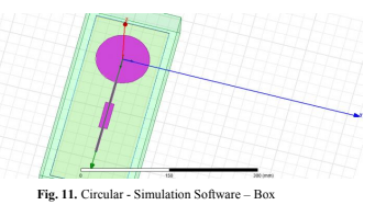
Similarly to what occurs in rectangular geometry, the simulation procedures for the circular patch antenna are quite similar. Fig. 11 (Circular – Simulation Software – Box) then shows the circular antenna design, Fig. 12 (Circular – Simulation Software – Return Loss) displays the return losses for different frequencies, and Fig. 13 (Circular – Simulation Software – Smith Chart) associates the reflection coefficients with the resonant frequency.
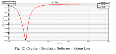
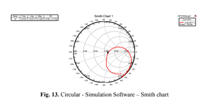
Note that, in this case, on the Smith Chart, you can associate the reflection coefficients present
according to the resonant frequency. This involves considering a null coefficient at the center of the circle and values increasing as you move away from the assumed point toward the center.
C. Fractal Order Variation: Sierpinski Carpet
Comparisons were made between rectangular and circular geometries, setting the resonance
frequency at 915 MHz. To obtain the resonance frequency, empirical adjustments were made to the dimensions of the Microstrip Lines and the 1/4 Wave Transformer. This was necessary because the fractal dimensions followed multiple values of the rectangular geometry.
For the fractal antenna design, only the internal rectangles were removed from order zero to order three. This alteration in resonance required different impedance matching for each order of fractals. However, the Y0 values remained almost unchanged. This is because the Y0 recess helps adjust the input impedance of the patch to 50 Ohms or values close to it, and the dimensions of the Microstrip Lines were chosen to be multiples of those calculated for the rectangular geometry.
The simulation of the first three orders of the fractal involved filling a rectangle measuring 78.71
mm x 99 mm, with the same line thickness but varying the total length. This helped determine the reflection coefficient at the input port, resulting in antennas of different fractal orders. The simulations were conducted using software design toolkit, producing the rectangular microstrip antenna as a reference point. Since there was no iterative process at this stage, the antenna was considered to be of Zero Order Sierpinski carpet fractal geometry. The dimensions of the fractals closely followed those of the rectangular geometry, with the Microstrip Line dimensions being proportional and multiples of the rectangular values. Subsequent
refinements were made in Ansys HFSS software simulations to fine-tune the Return Loss with the Resonance Frequency.
- Zero Order Fractal Geometry
Similar to the analysis conducted for the rectangular geometry.
- Order One Fractal Geometry
The rectangular-shaped patch is divided into nine identical rectangles, and subsequently, the central rectangle is eliminated. This process results in a microstrip antenna with Order One Sierpinski carpet geometry and Simulation Software, as shown in Fig. 14 (Order One – Simulation software).
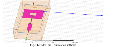
The simulation box met the minimum height of 10h, and the ground and substrate had their
minimum dimensions (110.00 x 220.00 mm), ensuring they did not touch the simulation box.
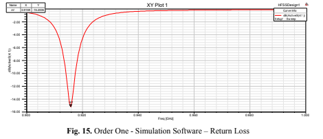
The reflection coefficient had a very low value, confirming a good impedance matching and a
resonant frequency precisely at the desired value, as shown in Fig. 15 (Order One – Simulation Software – Return Loss):
The Smith Chart, Fig. 16 (Order One – Simulation Software – Smith Chart), is a polar diagram of
the complex reflection coefficient. It combines the real and imaginary parts of a complex impedance on a
single graph, where the real part R can vary from 0 to infinity (∞), and the imaginary part X can span from (−∞, +∞).
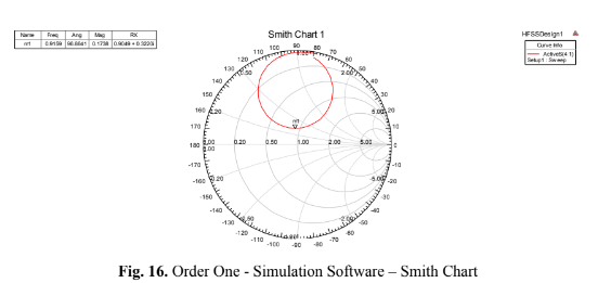
The chart also offers a method for illustrating scattering parameters (S parameters) and how these values correspond to practical circuit considerations and measurements.
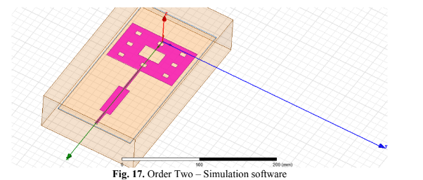
- Order Two Fractal Geometry
The aforementioned process applied to each of the eight new rectangles results in a microstrip
antenna with Level Two Sierpinski Carpet fractal geometry, as shown in Fig. 17 (Order Two – Simulation software).
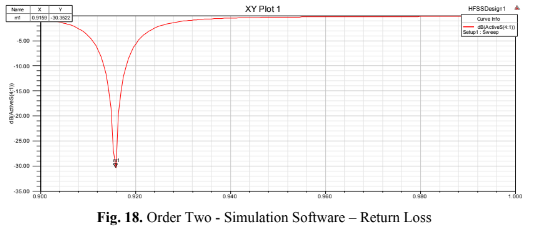
The reflection coefficient exhibited a very low value, confirming impedance matching and
resonance precisely at the desired frequency, as depicted in Fig. 18 (Order Two – Simulation Software – Return Loss)
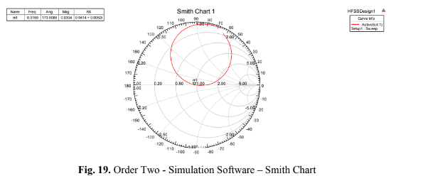
The red line in the chart represents the reflection coefficient at various frequencies. When it
intersects the center of the circle, it signifies that at that particular frequency, the reflection is null, and the return loss is minimized. This frequency marks the most significant resonance at which the antenna should be designed, as illustrated in Fig. 19 (Order Two – Simulation Software – Smith Chart).
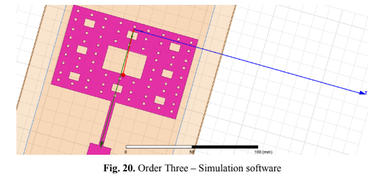
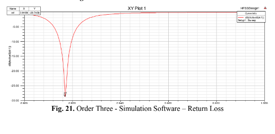
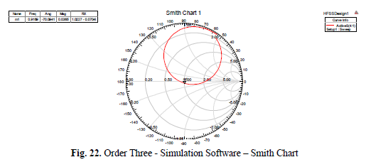
- Order Three Fractal Geometry
Similarly to what occurs in fractal geometries of orders 1 and 2, Fig. 20 (Order Three – Simulation
software), 21 (Order Three – Simulation Software – Return Loss), and 22 (Order Three – Simulation
Software – Smith Chart), respectively with the Geometry, Return Loss and Smith Chart, show the results obtained under the same conditions for the fractal geometry of order 3.
V. PATCH ANTENNA CONSTRUCTION
The antenna design was based on the Sierpinski Carpet Fractal. After defining the operating
frequency as 915 MHz, in alignment with the frequency used for RFID devices in Brazil and similar to those used in other countries for the same purpose, the patch antennas were constructed. These antennas were developed using a combination of mathematical principles, software simulations, and theoretical analyses. Empirical adjustments were introduced as needed to bring the simulated results into closer alignment with the real-world performance of each antenna. This allowed for the measurement of the actual operating frequency and reflection characteristics for each antenna. Additionally, through reverse engineering, it became possible to determine the electrical permittivity of the substrate. However, it’s important to note that this value is only accurate after conducting the necessary tests.
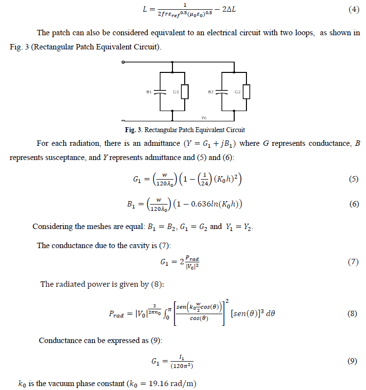
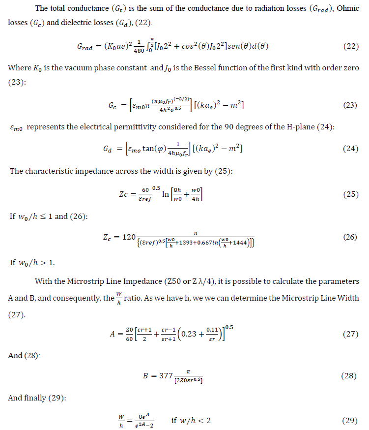
For the impedance matching from the antenna feed to the patch’s edge we used a generic expression (35), which is a representation of impedance along a transmission line, without accounting for losses.
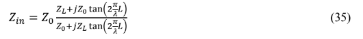
ZL represents the impedance at the end-load of the antenna, and Z0 refers to the microstrip line. The assembly was constructed using a 50 Ohm line with a length equal to half the wavelength.
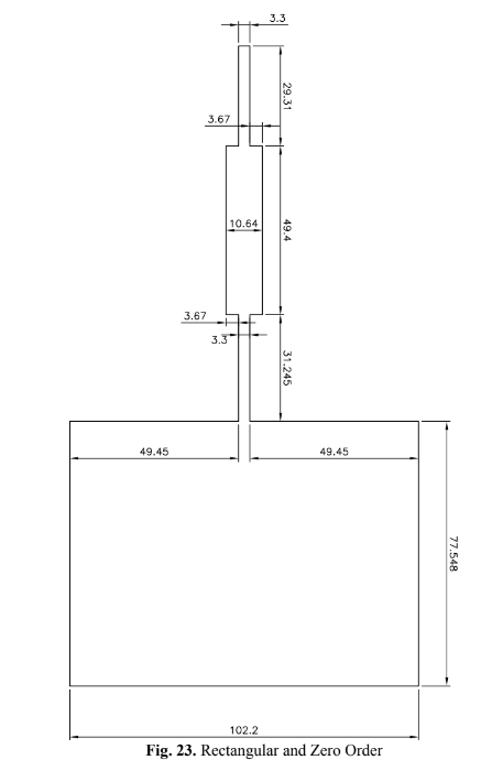
A. Rectangular and Zero Order Fractal
The microstrip line is defined by calculating the patch dimensions and assembling the antenna in the software. It is possible to calculate the value of Z_patch using Equation (35). To simplify, the length of the microstrip line is set to half the wavelength. The Zin given on the Smith Chart corresponds to the Z_patch itself (multiplied by 50 to account for normalization). Subsequently, the width of the 50 Ohm line can be calculated. Fig. 23 (Rectangular and Zero Order) shows a zero-order rectangular antenna.
For impedance matching, the quarter-wave transformer can only be matched to a resistive load. This length, denoted as ‘L’ of the microstrip line, transforms Zin into a real number. The calculations fororder one, two, and three fractals follow the same principles, involving iterations, and are summarized in Fig. 24 (Parameters Calculated for Patch Modeling. Sumarized results for one, two, and three fractal antennas).
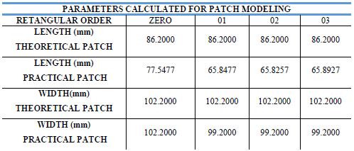
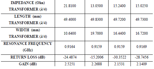
Fig. 24. Parameters Calculated for Patch Modeling.
Sumarized results for one, two, and three fractal antennas.
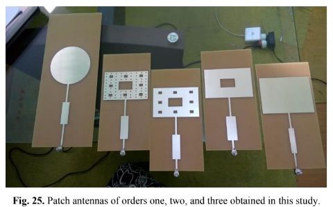
The Fig. 25 (Patch antennas of orders one, two, and three obtained in this study) shows an image of the manufactured patch antennas.
B. Analysis of Resonance Frequencies From 1.0 to 5.0 GHz – Ansys HFSS Software
For the manufactured antennas, a frequency sweep was performed, and the following resonant
responses were obtained, as shown in Fig. 26 to 30, respectively in Circular, Order Zero, Order one, Order two and Order three:
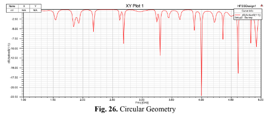
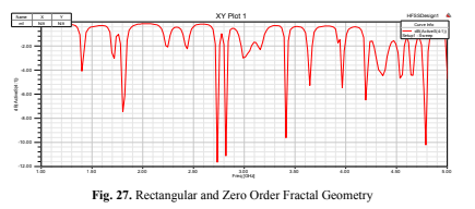
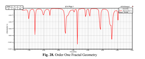
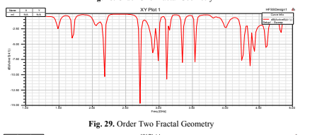
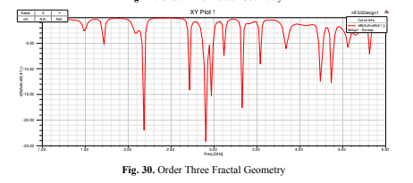
These findings demonstrate the unique behavior of Fractal antennas compared to traditional
geometries.
The analysis of the responses reveals the distinctions between Fractal antennas and traditional geometries:
- Resonant Frequencies: There is no linear increase in the number of resonant frequencies as the Fractal
Order is incremented. Resonance is defined by the presence of at least one amplitude below -10 dB.
Notably, in Order Three, more resonant frequencies were observed compared to other orders. - Return Loss: Increasing the Fractal Order leads to reduced return loss due to decreased reflections. As the
order iterates, the amplitude approaches levels lower than -10 dB at the resonant frequency with improved
impedance matching. In the case of Circular geometry, similar results were achieved, with a consistent
reduction in return loss as the order increased. However, the specific resonant frequencies varied across
orders. - Bandwidth: An increase in bandwidth was not directly proportional to the order of the Fractal. Bandwidth
measurements, which are based on frequency and encompass frequencies below -10 dB reflection, did not
exhibit a straightforward correlation with higher Fractal orders.
B. Measurements with VNA (Vector Network Analyser)
The manufactured antennas underwent laboratory testing using a VNA for the analysis of resonant frequencies, losses, and impedance matching (reflection factor).
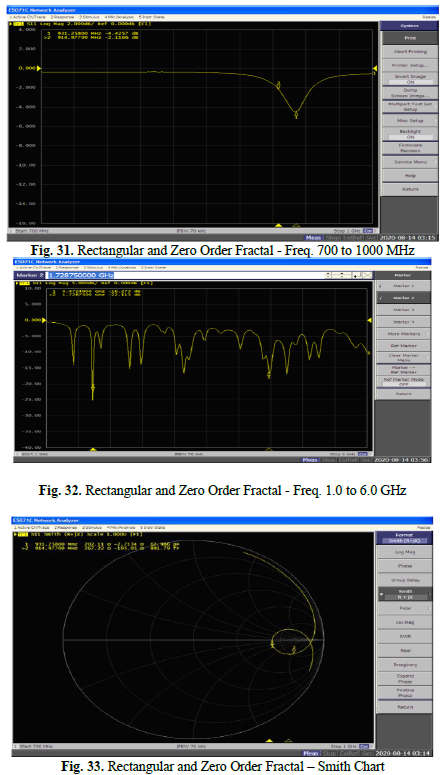
B.1. Rectangular and Zero Order Fractal Geometry
In the analysis of rectangular geometry and zero-order fractal geometry, we can observe the
following results:
Fig. 31 (Rectangular and Zero Order Fractal – Freq. 700 to 1000 MHz) illustrates the measured
resonant frequencies, revealing a minor deviation from the desired resonance frequency and a significant return loss. This return loss could be improved through enhanced impedance matching, with the frequency of approximately 931 MHz exhibiting a -4.5 dB return loss. Fig. 32 (Rectangular and Zero Order Fractal – Freq. 1.0 to 6.0 GHz) shows a broader frequency sweep, ranging from 1.0 to 6.0 GHz, enabling a comprehensive analysis of resonant frequencies. Notably, at the frequency of 1.72 GHz, excellent impedance matching was observed. Fig. 33 (Rectangular and Zero Order Fractal – Smith Chart) provides a graphical representation of the relationship between order values and return loss values with Smith Chart, we can associate reflection coefficients with the resonance frequency. It’s evident that lower order values
result in lower return loss values. These values are critical for assessing the antenna’s performance, with a return loss below -10 dB being the benchmark. The lower the return loss, the more feasible it is to implement the antenna for a particular frequency.
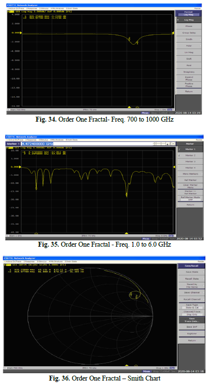
B.2. Order One Fractal
In this case, Fig. 34 (Order One Fractal- Freq. 700 to 1000 GHz) displays the resonant frequencies, which exhibit a slight deviation from 915 MHz. However, the return loss was high, signifying a suboptimal impedance match at this frequency (approximately 925 MHz with -2.5 dB). Upon closer examination of Fig. 35 (Order One Fractal – Freq. 1.0 to 6.0 GHz), we can analyze the resonant frequencies across a broader scanning range. A good impedance match was observed at the 4.47 GHz frequency. By plotting the Smith Chart, as depicted in Fig. 36 (Order One Fractal – Smith Chart), we can associate reflection coefficients with the resonance frequency. The chart assumes a null coefficient at the circle’s center, with values increasing as you move away from the assumed point towards the center. In this case, it is evident that the
reflection was somewhat distant from the center, indicating that the minimal reflection did not achieve a satisfactory value.
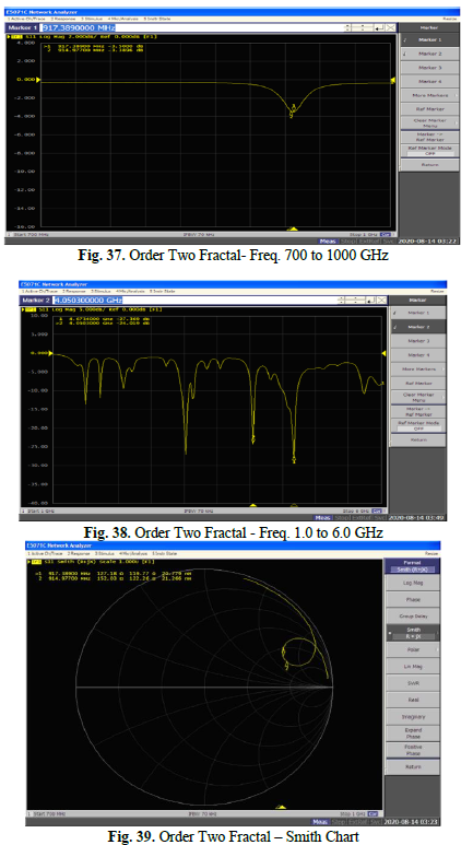
B.3. Order Two Fractal
The analysis to be conducted in this case should closely resemble that of fractal order one. Fig. 37 (Order Two Fractal- Freq. 700 to 1000 GHz) reveals a resonant frequency at 917 MHz with a return loss of 3.5 dB. When scanning frequencies across a broader range, from 1.0 to 6.0 GHz, Fig. 38 (Order Two Fractal
- Freq. 1.0 to 6.0 GHz) illustrates several resonant points, demonstrating a good impedance match at the 4.67 GHz frequency. Fig. 39 (Order Two Fractal – Smith Chart) displays the results of the reflection coefficient plotted on the Smith Chart.
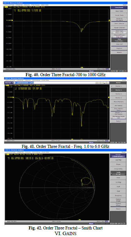
B.4. Order Three Fractal
Regarding the Order Three fractal, the analysis performed is the same. Fig. 40 (Order Three Fractal- 700 to 1000 GHz) displays the measured resonant frequencies, Fig. 41 (Order Three Fractal – Freq. 1.0 to 6.0 GHz) shows the analysis of resonant frequencies over a broader range, and Fig. 42 (Order Three Fractal
– Smith Chart) presents the results of the reflection coefficient plotted on the Smith Chart. A sharp return loss is observed at 4.6 GHz, with the second most pronounced loss at 4.1 GHz, indicating low reflection and good impedance matching, though not at the desired frequency. It is also worth noting that close to 4.1 GHz, there is a considerable bandwidth with return loss values below -10 dB, providing a wide working frequency range.
In practice, gain measurements were conducted in two stages: first, using a Vector Network
Analyzer (VNA) for a single connection, where power was transmitted through a 50 Ohm cable.
Subsequently, measurements were taken in an Anechoic Chamber, which necessitates both a transmitting antenna (the antenna under evaluation) and a receiving antenna (in this case, a Yagi-Uda antenna, shown in yellow in Fig. 43-Anechoic Chamber-front and Fig. 44-Receiving antenna Yagi-Uda in yellow-back). The Yagi-Uda antenna received the electromagnetic signals emitted by the antenna under evaluation, with a predefined power, and the distance between them was set at 3 meters for optimization. The antenna under evaluation was positioned on a rotating table equipped with a stepper motor, allowing us to assess its signal emission at various angles. Meanwhile, the receiving antenna remained stationary. This method was chosen because gains vary with changing angles. Subsequently, the collected data were used to evaluate gains in both the vertical and horizontal planes. The measurements were taken at 360o to ascertain the complete gains in these planes. The Fig. 45 (Equipment) show the types of equipment that allows controlling the power supplied to the antennas to be evaluated.
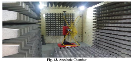
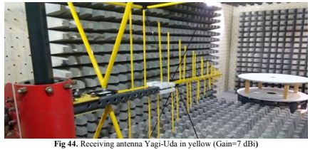
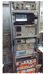
Fig. 45. Types of equipment that allows controlling the power supplied to the antennas to be evaluated, the angular speed of the rotatory table, manipulating the angulation of the Yagi-Uda receiving antenna, controlling the internal temperature and the humidity
level inside the anechoic chamber.
The gain in dBi can be calculated by the following expression (36):
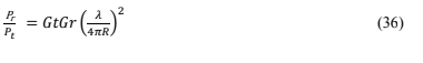
Where,
Pr – represents the received power (Obtained at each point of the radiation diagram).
Pt – represents the transmitted power (The power input into the RF Generator, which is -45 dBm).
Gr – represents the receiver antenna gain (Yellow Antenna Gain at 915 MHz, which is 7 dBi).
Gt – represents the desired gain of the Fractal antenna.
λ – represents the wavelength of 915 MHz in air.
R – represents the distance between the Antennas (3m).
C. Antenna Gain
The Table II, depicted in Fig. 46 (Gains Measured in Anechoic Chamber), summarizes the obtained gain results from the anechoic chamber.
TABLE II
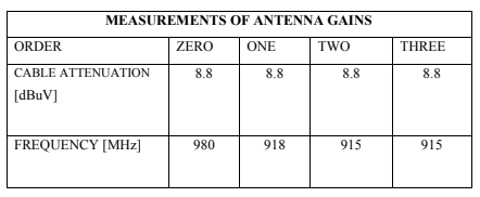
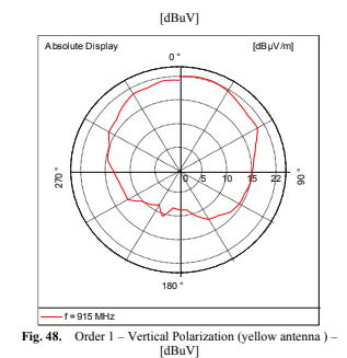
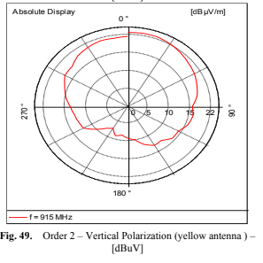
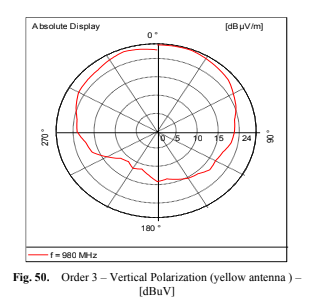
When the antenna on the turntable transmits at a specified power, the receiving antenna captures the waves based on this angle (measured in amplitudes, shown in the red graph). To assess how the antenna’s radiation behaves in both the vertical and horizontal planes, the amplitude values (magnitude of each vector) are examined in dimensions (x, y, z).
To determine the angle at which the maximum amplitude occurs within 360 degrees, the vector intensity in each plane is evaluated, and the highest value is selected as the antenna’s gain. The magnitude of the irradiation intensity is compared in the vertical and horizontal planes, and the plane with the maximum value represents the antenna’s overall gain. For amplitude values with the envelope depicted in red on the graphs below, the Friis Formula (Equation 36) is applied to calculate the Received Power (Pr) in [dBuV].
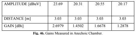
Additionally, antenna directivity can be analyzed. If the radiation is evenly distributed over 360
degrees, the antenna scatters the signal in all directions and exhibits low directional performance. This angle is defined by the vectors perpendicular to each antenna’s surface. In the case of patch antennas, it lies within the same plane, while for Yagi-Uda antennas, it aligns with the antenna’s central axis. The graphs Fig. 47 (Vertical Polarization (yellow antenna) [dBuV]-order zero), 48 (Vertical Polarization (yellow antenna) [dBuV]-order one), 49 (Vertical Polarization (yellow antenna) [dBuV]-order two) and 50 (Vertical Polarization (yellow antenna) [dBuV]-order three), respectively order zero, one, two and three, depict the transmission and reception signal strength in relation to the angle between the transmitting and receiving
antennas.
VII. ANALYSIS OF RESULTS
The antennas were designed to operate at a resonant frequency of 915 MHz, and their dimensions were determined through theoretical calculations. The impedance matching was based on both theoretical considerations and empirical adjustments, particularly in the design of the 1/4 wave transformer. Simulations indicated close resonance to the desired frequency and nearly perfect impedance matching, with a return loss below -10 dB and a Smith Chart close to its center.
In laboratory testing, impedance matching was nearly perfect, but there was a slight deviation in resonance frequency. These antennas provided valuable data for calculating the substrate’s electrical permittivity, which could only be determined empirically.
While the patch impedance was assumed to be resistive, it required practical adjustments to achieve the desired characteristics, including the Y0 recess for the rectangular antenna. Fractal antennas lack a theoretical basis for calculating their impedances and dimensions, necessitating empirical adjustments.
The main challenge was achieving impedance matching with a 1/4 wave transformer. While the patch impedance was intended to be resistive, this factor was not confirmed, and practical adjustments were necessary. Equation (35) was used to model impedance matching algebraically, enabling the calculation of patch impedance and the adjustment to make it resistive, as well as determining the dimensions of the 1/4 wave transformer.
The simulations demonstrated good impedance matching and precise resonance frequencies up to the third decimal place. However, bench tests revealed some discrepancies, with the impedance matchingnot aligning perfectly with the simulation. Despite these divergences, the assembled antennas generally met their design specifications.
In the case of fractal antennas, an increase in the fractal order resulted in decreased return loss at resonant frequencies. However, it was observed that different antennas did not resonate at the same frequencies. Additionally, order three fractals exhibited a significantly higher number of resonant frequencies compared to others, suggesting that increasing the fractal order could lead to more resonant frequencies.
Regarding bandwidth (the range of frequencies with a return loss below -10 dB), there was no linear increase with higher fractal orders. Nevertheless, there was a trend for non-resonant frequencies adjacent to the resonant ones to exhibit a return loss below zero, especially in higher-order fractals compared to traditional geometries. This suggests that fractals could potentially enhance bandwidth as iterations increase due to the adjacent frequencies becoming resonant.
VIII. CONCLUSION
Fractals offer the potential to expand both bandwidth and the number of resonant frequencies,
making them well-suited for Fifth Generation (5G) applications that demand a wide and varied operating frequency range. These geometric structures provide exceptional flexibility by definition, generating a diverse array of resonant frequencies. This adaptability allows antennas to be customized for specific project requirements.
Fractals also facilitate adjustments in shape and material quantities to match the desired operating frequency, resulting in reduced return loss and reflections in transmission lines. This optimization leads to improved signal transmission between distant points in space, enhancing overall performance.
AKNOWLEGMENT
This study was conducted within the framework of the Verbena V9 project, which is partially
funded by CAPES and involves collaboration with NC – LabTelecom. Special appreciation goes to the colleagues at LabTelecom for their valuable contributions to enhancing the quality of this paper. Additionally, we extend our thanks to the Academic Publishing Advisory Center (Centro de Assessoria de Publicação Acadêmica – CAPA) at the Federal University of Paraná for their assistance with English language editing.
REFERENCES
[1] F. Abdelhak, F. Najib, S. Noureddine, and G. Ali, “Analysis and Design of Printed Fractal Antennas by Using an Adequate
Electrical Model,” Int. J. Commun. Networks Inf. Secur., vol. 1, no. 3, pp. 67–72, 2009.
[2] Batra, Rahul S. Sange, Dipika S. Zade, P.L. “Design of modified geometry Sierpinski carpet fractal antenna array for
wireless communication”. IEEE International Advance Computing conference (IACC). 2013.
[3] L. DEBNATH, “A Brief Historical Introduction to Fractals and Fractal Geometry,” Int. J. Math. Educ. Sci. Technol., vol.37:1, pp. 29–50, 2006, doi: 10.1080/00207390500186206.
[4] M. S. Fairbanks, D. N. McCarthy, S. A. Scott, and S. A. B. R. P, “Fractal electronic devices: simulation and Implementation,” Nanotechnology, vol. 22, no. 36, 2011.
[5] F. A. Ghaffar, “Design of LTCC Based Fractal Antenna,” KAUST Research Repository., 2010.
[6] Cao, Thanh Nghia. Krzysztofik, Wojciech J. Design of multiband sierpinski farctal carpet antenna array for C-band. IEEE
International Microwave and Radar Conference (MIKON). 2018. Conference (MIKON). 2018.
[7] A. Trikolikar and S. Lahudkar, “A Review on Design of Compact Rectenna for RF Energy Harvesting,” in 2020 International Conference on Electronics and Sustainable Communication Systems – ICESC, 2020, pp. 651–654, doi: 10.1109/ICESC48915.2020.9155984.
[8] Anuradha, S. Buravalli, Manasa. Kumar, Tejaswini. Shilpa, G. D. Simulation Study of 2×3 Microstrip Patch Antenna Array for 5G Applications. IEEE 5th Internacional Conference on Computing, Communication and Security (ICCCS). 2020.
[9] M. A. Darmawan and U. Khayam, “Design, simulation, and fabrication of second, third, and forth order Hilbert antennas as ultra high frequency partial discharge sensor,” in Proceedings of the Joint International Conference on Electric Vehicular Technology and Industrial, Mechanical, Electrical and Chemical Engineering (ICEVT & IMECE), 2015, pp. 319–322, doi: 10.1109/ICEVTIMECE.2015.7496707.
[10] E. Sama, M. Ameen, and O. Sattar, “Design and Simulation of Microstrip Patch Antenna for 5G Application using CST Studio,” Int. J. Adv. Sci. Technol., vol. 29, pp. 7193–7205, 2020.
[11] P. Namdeo, N. Agrawal, P. Yadav, and R. Vishwakarma, “Design and Analysis of Sierpinski Carpet Fractal Antenna,” ISSN 2321-2004 ISSN 2321-5526 Int. J. Innov. Res. Electr. Electron. Instrum. Control Eng., vol. 3, no. 5, 2015.
[12] K. Sing, V. Grewal, and R. Saxena, “Fractal Antennas: A Novel Miniaturization Technique for Wireless Communications,” Int. J. Recent Trends Eng., vol. 2, no. 5, pp. 172–176, 2009.
[13] J. Colaco and R. B. Lohani, “Design and Implementation of Microstrip Circular Patch Antenna for 5G Applications,” in 2020 International Conference on Electrical, Communication, and Computer Engineering (ICECCE), 2020, pp. 1–4, doi: 10.1109/ICECCE49384.2020.9179263.
[14] Aswoyo, Budi. Putra, Anggara Hadhy. High Gain Microstrip Square Patch Array Antenna 4X4 Element 2.3 GHz for 5G Communication in Indonesia. IEEE Enternational Electronics Symposium (IES). 2021.
[15] Kalaivarasan, R. Nagarajan, G. Seenuvasamurthi, S. The state of the art design methodology of sierpinski carpet fractal structures in microstrip patch antenna. IEEE 7th International Conference on Computing in Engineering e Technology (ICCET 2022). 2022.
[16] I. Maxim, “Impedance Matching and the Smith Chart: The Fundamentals,” http://rf-
opto.etti.tuiasi.ro/docs/files/tutorial.pdf 2002.
1 Department of Electrical Engineering, Federal University of Paraná-UFPR, Curitiba, Paraná, Brazil. nakaronaldo2020@gmail.com, pedropompilio@ufpr.br, clbtx@uol.com.br, brunoricobom@hotmail.com, tertuliano@ufpr.br;
* Principal Author;
†The contributions of these authors are equal in this work.