REGISTRO DOI: 10.5281/zenodo.8287885
Rafael Oliveira Ribeiro
Abstract
This paper demonstrates how to obtain three-dimensional (3D) information based on pairs of images that capture approximately the same scene, considering two distinct cases. In the first case both images are perfectly rectified, whereas in the second case the cameras’ image planes are not parallel to each other, i.e., there exists a vertical disparity between the images. Dense depth maps are computed for both cases and compared with ground truth information when available. Additionally, triangulation is used to compute sparse 3D reconstruction of an object for selected points. The computation of dense depth maps used a modified version of the Semi-Global Matching (SGM, [4]) algorithm available in the OpenCV [1] library, augmented with post-processing techniques. Parameters for the modified SGM algorithm and for the post-processing stage were found by global optimization on 21 scenes from the 2014 Middlebury datasets [8]. This optimization strategy achieved significant improvement in the computation of dense depth maps when compared with default or recommended parameters for the SGM and postprocessing filters. A trade-off between speed and accuracy in the post-processing stage was demonstrated.
1. Introduction
This report focuses on the topic of 3D reconstruction based on stereo vision and it has three objectives: i) computation of dense depth maps from rectified stereo images; ii) computation of dense depth maps from non-rectified stereo images; and iii) sparse 3D reconstruction of an object with inference of its real-world dimensions.
All these objectives depend on locating, in each image, the corresponding projections (i.e., the pixels) of each point of the scene that is captured in both images. Information on the relative position and orientation of the cameras, as well as their intrinsic parameters, are also necessary. The search for correspondences in both images can be optimized with the use of epipolar geometry, which reduces the search space from 2D to 1D.
In the simplest case, the image planes from both cameras coincide and there is only horizontal displacement between the cameras’ centers. In this case, the epipolar lines are parallel to each other and horizontal. Thus, the search for corresponding pixels can be restricted to a line with the same y-coordinate in both images. An additional constraint on the maximum disparity can further reduce the search space.
In cases where the image planes are not in this relative position, both images can be firstly projected to a common plane, such that the epipolar lines are parallel and have the
same y-coordinate – a process called stereo rectification. One can then proceed in the same way as in the previous case.
According to the taxonomy and categorization presented in [7], stereo matching algorithms generally perform some subset of the following four steps: 1. matching cost computation; 2. cost (support) aggregation; 3. disparity computation and optimization; and 4. disparity refinement.
Under this taxonomy, the disparity computation and optimization step can be classified between local and global methods. In local methods, after the computation and aggregation of the matching costs, the pixel associated with the smallest cost is chosen as the match, following a “winner-take-all” strategy. On global methods, matches are determined in a way to minimize some cost function that is computed globally over the image.
The algorithm used in this work (SGM) applies a mix of local and global strategies: the matching cost is computed for each pixel, but this cost is computed after aggregating along multiple directions in the image. The OpenCV implementation of SGM has some differences to the original algorithm, most notably the use of block matching (although pixel matching is possible), a different cost function and the inclusion of pre- and post-filtering.
2. Dense depth maps from rectified stereo images
In the case of rectified stereo images, all disparities lie along a horizontal line and their value is inversely proportional to the depth (distance) to the cameras. For the conversion of disparity values to distances, it is also necessary to know the cameras’ focal distance f and the baseline (the distance between the cameras’ centers). The doffs parameter (x-difference of principal points) must also be included in the conversion, which can be achieved by the formula Z = baseline∗ f/(disparity+dof fs).
In this section we detail the computation of disparity and depth maps for the datasets Playtable and Jadeplant, from the 2014 Middlebury stereo datasets [8]. See Figure 1.
2.1 Methodology
The Semi-Global Match algorithm was chosen because it was readily available in the OpenCV library and its implementation allows for a variety of parameters to be explored. Also, there are at least ten submissions to the Middlebury Stereo Evaluation, v. 3, that are based on this algorithm, so the results of this paper could also be evaluated against such submissions.
Post-processing the disparity maps was necessary to handle invalid pixels (corresponding to points that are captured by only one image), noise and artifacts. Two techniques were studied: a simple morphological (Morph) close operation, aimed to “fill the holes” of invalid pixels, and a more elaborate technique, based on a Weighted Least Squares (WLS) filter, with the use of left-right consistency check of disparity maps.[1]
The metric used for evaluation was the bad2.0, which is the percentage of pixels with disparity error greater than 2.0.
After an initial assessment of parameters of the SGM algorithm and of the two postprocessing strategies, it became clear that the best parameters for one dataset were not optimal for the other. This motivated a more thorough investigation of the parameters, which was carried out in the form of a grid search, performed on the 21 remaining datasets from Middlebury that have ground truth available.
The parameters considered for optimization are listed in Table 1, along with the algorithm in which it is used and the values tested for each parameter. The combination of bold values minimizes the average of the bad2.0 metric in the 21 datasets.
Figure 1: The two datasets used for this part of the paper. Left images (above) and ground truth disparity maps (below). Lighter tones correspond to higher disparities.
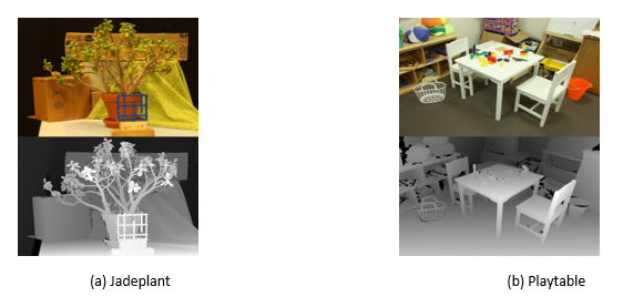
Table 1 – Parameter optimization for SGM, WLS and Morph.
Parameter Algorithm Values blockSize SGM 3, 7, 15 disp12MaxDiff -1, 0, 1 uniquenessRatio 0, 10, 20 speckleWindowSize 0, 50, 100 speckleRange 0, 1 Lambda WLS 40, 80, 200, 800, 8000, 80000 SigmaColor 0.4, 0.8, 1.2, 2.0 kernelSize Morph 5, 15, 25, 45, 75
The optimization was carried out in two stages: the parameters of SGM were optimized first and kept constant for the optimization of the post-processing stage. WLS and Morph were optimized in a mutually exclusive manner: either one or the other is used.
In the OpenCV implementation of SGM, only pixels with x-coordinate greater than the maximal disparity are considered, if the left image is the reference. To mitigate this, images were left- or right-padded prior to the computation of disparity maps. The computed disparity maps were then cropped to remove the padding areas.
2.2 Results
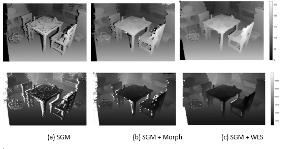
The parameters optimized according to the previous section were used to process the Jadeplant and Playtable datasets and the results are summarized in Table 2. Figures 2 and 3 show the corresponding disparity and depth maps for the two datasets.
Table 2 – Trade-off between accuracy and speed for the post-processing alternatives.
Dataset Pipeline timing (s) bad2.0 (%) Jadeplant SGM 12.6 ±0.24 44.56 SGM + WLS 25.5 ±0.38 38.92 SGM + Morph 13.0 ±0.08 42.82 Playtable SGM 4.5 ±0.09 30.78 SGM + WLS 9.4 ±0.22 26.46 SGM + Morph 4.6 ±0.11 28.54
Figure 2: Disparity (top) and depth maps (bottom) for the Jadeplant dataset.

3. Dense depth maps from non-rectified stereo images
In this section we demonstrate the computation of dense depth and disparity maps for two images from the 3D Photography Dataset, by Y. Furukawa and J. Ponce[2].
3.1 Methodology
The main difference from the methodology described in Section 2.1 is related to rectifying both images prior to computing the disparity and depth maps.
Figure 3: Disparity (top) and depth maps (bottom) for the Playtable dataset.
The rectification can be performed with the use of homographies derived from the fundamental matrix (F). According to [3], F is the algebraic representation of the epipolar geometry and it has the property that, for corresponding points x and x0, xFx0 = 0.
This relation allows one to derive F and perform the rectification without knowing the camera parameters. This possibility is explored in this work by finding corresponding points with the use of Scale Invariant Feature Transform (SIFT, [5]), matching these points with Fast Approximate Nearest Neighbors [6], and computing F using a Random Sample Consensus (RANSAC, [2]) strategy – see Figure 4(a).
Figure 4: Stereo rectification using point correspondences.
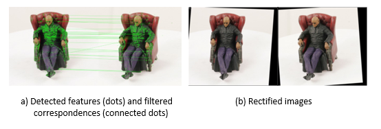
After the Fundamental matrix is obtained, homographies are computed for the reprojection of each image. The reprojected images are shown in Figure 4(b).
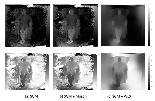
After rectification, the computation of disparity and depth maps are done in the same way as in the previous section. Since there is no ground truth available for this dataset, the disparity maps were only visually evaluated. The optimal values for SGM from the previous section were used, but with different values for the WLS filter (SigmaColor = 1.8 and Lambda = 8000) and for Morph (kernelSize = 7).
3.2 Results
Figure 5 shows the disparity and depth maps obtained with the use of the optimal parameters found in Section 2 and with different parameters for the WLS filter and a pre-process stage.
Figure 5: Disparity (top) and depth maps (bottom) for the Morpheus images.
4. Sparse 3D reconstruction
The objective of this part is to estimate the dimensions of an object that is captured by two distinct cameras and compute the dimensions of a cube into which the object could be fitted.
Dense 3D reconstruction could be used if more views of the object were captured, but with only two views, some parts of the object were never captured. Therefore, a simpler approach to recover the 3D coordinates of only some specific points of the object was chosen. These coordinates and some assumptions about the shape of the object were used to compute the volume of the cube into which the object could be fitted.
4.1 Methodology
To recover the 3D coordinates of points captured by two calibrated cameras with known pose, i.e., with known intrinsic and extrinsic parameters, a triangulation method can be used.
Considering X a point in 3D space, it will be projected by one camera with projection matrix P as xT = PX, and by the other camera with projection matrix P’ as x’T = P’X. With these projections and calibration information of both cameras, one can compute two rays into space and the problem to locating the point X in space becoming one of finding the intersection of both rays.
In the absence of noise, this would yield an exact solution. But when noise is factored in, an exact solution is no longer available and a solution can be computed by expressing the correspondences as a linear system of equations in the form of AX=0, with the matrix A
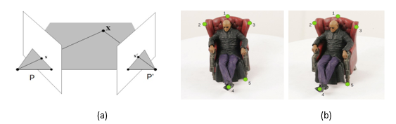
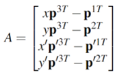
Figure 6: (a) Geometry of triangulation, adapted from [3], with two calibrated cameras, P and P0, and projections x and x0 of the point X; (b) images used for this part of the paper, with the points of interest marked.
having the form of:
where piT is the i-th line of matrix P, and solving for X using the singular value decomposition of A. The camera matrices were obtained by the formula P = K[R|t], where K, the intrinsic matrix, R, the rotation matrix, and t, the translation vector of the camera center, were build using the appropriate elements from the calibration data for each image.
After computing the 3D coordinates of the five points marked in Figure 6(b), we proceed as follows to obtain the dimensions of a cube that could encompass the object: one dimension (width) of the cube is the euclidean distance between points 2 and 3; the second dimension (height) is the difference between the Z-coordinates of points 1 and 5; and the third coordinate (depth) is the euclidean distance between point 4 and the projection of point 1 to the same Z-coordinate of point 4.
.2 Results
The 3D coordinates obtained for points 1, 2, 3, 4 and 5 were [93, 144, 113.1], [71.2, 103.1,101], [134.1, 162.5, 99.3], [185, 54.2, 17.8] and [156.9, 122.3, -7.2], which results in a cube of dimensions 47.9 mm x 120.3 mm x 128.6 mm.
5.Discussion and conclusion
From the computation of disparity and depth maps (sections 2 and 3), it became clear that the parameters for the stereo matching algorithm and for post-processing are, to some extent, specific to the content and size of the images. Algorithms that can take these differences into account and automatically adjust its parameters may be an alternative to overcome this specificity observed in this paper. Also, a trade-off between speed and accuracy was observed, which should be taken into account depending on the application.
References
G. Bradski. The OpenCV Library. Dr. Dobb’s Journal of Software Tools, 2000.
Martin A. Fischler and Robert C. Bolles. Random sample consensus: A paradigm for model fitting with applications to image analysis and automated cartography. Commun. ACM, 24(6):381–395, June 1981. ISSN 0001-0782. doi: 10.1145/358669.358692. URL https://doi.org/10.1145/358669.358692.
Richard Hartley and Andrew Zisserman. Multiple View Geometry in Computer Vision. Cambridge University Press, 2 edition, 2004. doi: 10.1017/CBO9780511811685.
H. Hirschmuller. Stereo processing by semiglobal matching and mutual information. IEEE Transactions on Pattern Analysis and Machine Intelligence, 30(2):328–341, 2008. doi: 10.1109/TPAMI.2007.1166.
D. G. Lowe. Object recognition from local scale-invariant features. In Proceedings of the Seventh IEEE International Conference on Computer Vision, volume 2, pages 1150– 1157 vol.2, 1999. doi: 10.1109/ICCV.1999.790410.
Marius Muja and David G. Lowe. Fast approximate nearest neighbors with automatic algorithm configuration. In In VISAPP International Conference on Computer Vision Theory and Applications, pages 331–340, 2009.
Daniel Scharstein and Richard Szeliski. A taxonomy and evaluation of dense two-frame stereo correspondence algorithms. International Journal of Computer Vision, 47:7–42, 04 2002. doi: 10.1023/A:1014573219977.
Daniel Scharstein, Heiko Hirschmüller, York Kitajima, Greg Krathwohl, Nera Nešic,´ Xi Wang, and Porter Westling. High-resolution stereo datasets with subpixel-accurate ground truth. In Xiaoyi Jiang, Joachim Hornegger, and Reinhard Koch, editors, Pattern Recognition, pages 31–42, Cham, 2014. Springer International Publishing.
[1] This filter was implemented in the class https://docs.opencv.org/4.4.0/d9/d51/classcv_1_ 1ximgproc_1_1DisparityWLSFilter.html from the OpenCV library.
[2] The dataset is no longer available online, but a description can be found on https://web.archive. org/web/20170615075554/https://www.cse.wustl.edu/~furukawa/research/mview/ index.html
Filiação